Dynamic mesh tutorials
In this chapter we shall describe in detail the process of setup, simulation and post-processing for SedFoam test cases using dynamic meshes. All the tutorial cases are located in the tutorialsDyM directory.
Installation Prerequisites
Before launching any numerical simulation, make sure overSedDymFoam_rbgh is correctly installed and compiled:
First, download the the official SedFoam package:
git clone --recurse-submodules http://github.com/sedfoam/sedfoam
Compile the program by running Allwmake:
cd sedfoam
source $FOAM_ETC/bashrc # load the openfoam environment
./Allwmake
The program should compile without problems and the binary
overSedDymFoam_rbghand associated libraries should be available in the $FOAM_USER_APPBIN and $FOAM_USER_LIBBIN directories.
To take full advantage of SedFoam and be able to run the postprocessing scripts make sure Python is installed. Python usually comes pre-installed in Linux. However, if not installed or if you need a specific version, you can install Python with the following command:
sudo apt install python3
Further details can be found in section Installation .
FallingSphereOverset: Falling sphere in pure fluid using an overset approach
In this tutorial, we study the free fall of a sphere with a diameter settling in silicon oil using the overset approach. The experimental setup consists of a rectangular box measuring (click here to go to the article associated to this experiment) . The input parameters have been chosen to reproduce the experiments of a settling sphere at a Reynolds number equal to , where is the terminal velocity of the sphere. The numerical case can be found in the folder sedFoamDirectory/tutorialsDyM/FallingSphereOverset. This benchmark is inspired by the online tutorial of a settling sphere of OpenFOAM. The physical parameters are summarized in the following table:
| Properties | Value |
|---|---|
| Sphere density | |
| Fluid density | |
| Fluid viscosity | |
| Sphere diameter |
Mesh generation and setup
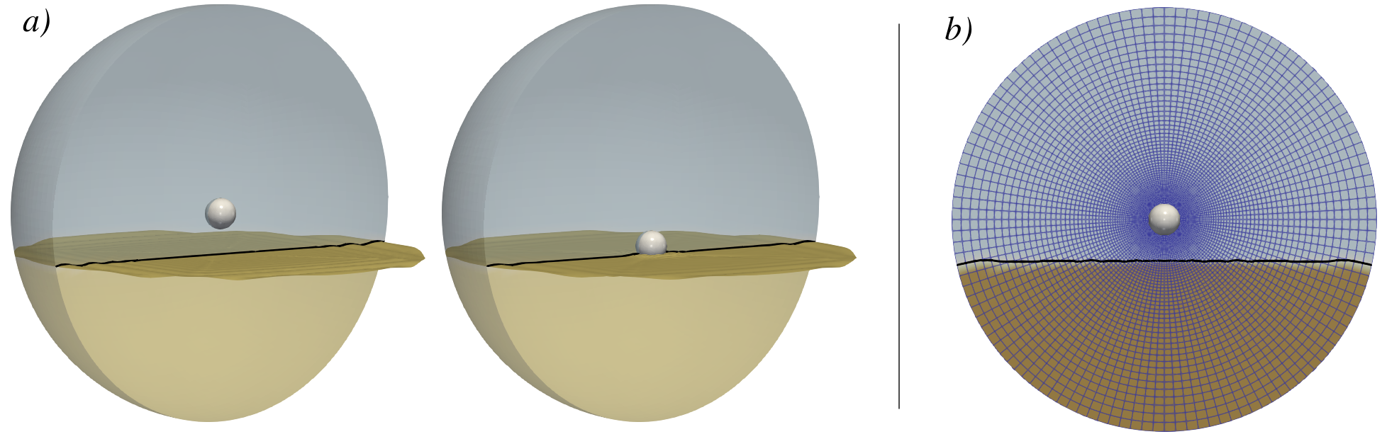
The numerical domain consists of two disconnected meshes. The background mesh, which remains static throughout the simulation, is a hexahedron with a side length of , while the overset mesh that moves relative to the background mesh is a hexahedron with a side length of . These meshes are illustrated in Figure 1
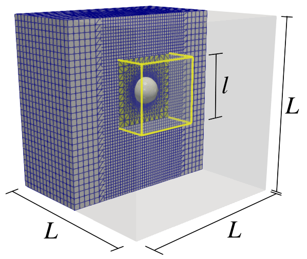
The overset mesh is generated by running the command blockMesh in the tutorialsDyM/FallingSphereOverset/sphereMesh folder. Then, the meshing utility snappyHexMesh is executed to generate a finer mesh near the spherical object. The meshing, refinement process and scale transformation are generated by running:
blockMesh
snappyHexMesh -overwrite
transformPoints -scale '0.0075'
Finally, topoSet needs to be executed to add the moving cells. Alternatively, one can execute *./Allrun.pre* in the tutorialsDyM/FallingSphereOverset/sphereMesh folder to generate the overset mesh.
Afterwards, we need to generate the background mesh and merge the two meshes. To do so, we will execute the *./Allrun.pre* command in the tutorialsDyM/FallingSphereOverset/sphereAndBackground folder. By running *./Allrun.pre* we are executing a sequence of several commands that we can break down here one by one to understand their meaning:
blockMesh
topoSet -dict system/topoSetDictR2
refineMesh -dict system/refineMeshDict2 -overwrite
The mesh is generated, and topoSet and refineMesh are called to refine the mesh along the vertical direction of the sphere trajectory. The refinement in this vertical region is carried out to reduce the interpolation errors between the background mesh and the overset mesh around the sphere. Then,
mergeMeshes . ../sphereMesh -overwrite
topoSet
The sphere is added into our setup and topoSet is executed to select cellSets for the different zones.
In the last part of Allrun.pre script, we create the initial time folder and use cellSets to write zoneID. Each cell zone, indicated in the zoneID field, should have a different zone id. In our case, there are two zones: the zoneID cells of the background mesh are set to 0 while zoneID cells belonging to the overset mesh are set to 1:
In the last part of Allrun.pre script, we create the initial time folder and use cellSets to write zoneID. Each cell zone, indicated in the zoneID field, should have a different zone id. In our case, there are two zones: the zoneID cells of the background mesh are set to 0 while zoneID cells belonging to the overset mesh are set to 1:
cp -r 0.orig 0
setFields
Dynamic mesh
Mesh changes are only possible if we have a file called dynamicMeshDict in the constant folder. Several mesh options and controls can be adjusted in the dynamicMeshDict dictionary. In this file we need to specify that the motion solver (in our case sixDoFRigidBodyMotionSedFoam), the patch where the 6DoF is acting, and set the moment of inertia and the apparent mass of the object. The 6DoF solver integrates the viscous, frictional, granular and excess of fluid pressure forces over the patch to get the velocity and displacement of the sphere.
/*--------------------------------*- C++ -*----------------------------------*\
| =========                 |                                                 |
| \\      /  F ield         | OpenFOAM: The Open Source CFD Toolbox           |
|  \\    /   O peration     | Version:  v2306                                 |
|   \\  /    A nd           | Website:  www.openfoam.com                      |
|    \\/     M anipulation  |                                                 |
\*---------------------------------------------------------------------------*/
FoamFile
{
    version     2.0;
    format      ascii;
    class       dictionary;
    object      motionProperties;
}
// * * * * * * * * * * * * * * * * * * * * * * * * * * * * * * * * * * * * * //

motionSolverLibs ( sixDoFRigidBodyMotionSedFoam );

dynamicFvMesh       dynamicOversetFvMesh;

dynamicOversetFvMeshCoeffs
{
}

motionSolver          sixDoFRigidBodyMotion;
accelerationRelaxation 0.4;

sixDoFRigidBodyMotionCoeffs
{
    patches         (sphere);
    innerDistance   100.;
    outerDistance   101.;

    accelerationRelaxation 0.4;
    accelerationDamping 0.4;

    //  mass reduced by Buoyancy: (rhosolid - rhofluid ) * VolumeSphere
    mass            2.65E-04;
    centreOfMass    ( 0 0 0 );
    momentOfInertia ( 4.45E-08 4.45E-08 4.45E-08);
    rho             rhoInf;
    rhoInf          970;
    g               (0 0 -9.81);
    report          on;
    reportToFile    on;

    solver
    {
        type Newmark;
    }
}
Computation launching
The simulations will run in parallel on 4 cores by executing the following commands at tutorialsDyM/FallingSphereOverset/sphereAndBackground folder:
decomposePar
mpirun -np 4 overSedDymFoam_rbgh -parallel > log.out&
One can skip all the previous steps and simply run the command *./Allrun* in the tutorialsDyM/FallingSphereOverset folder. It is worth mentioning that the output data will be stored in the tutorialsDyM/FallingSphereOverset/sphereAndBackground folder.
Post-processing using python
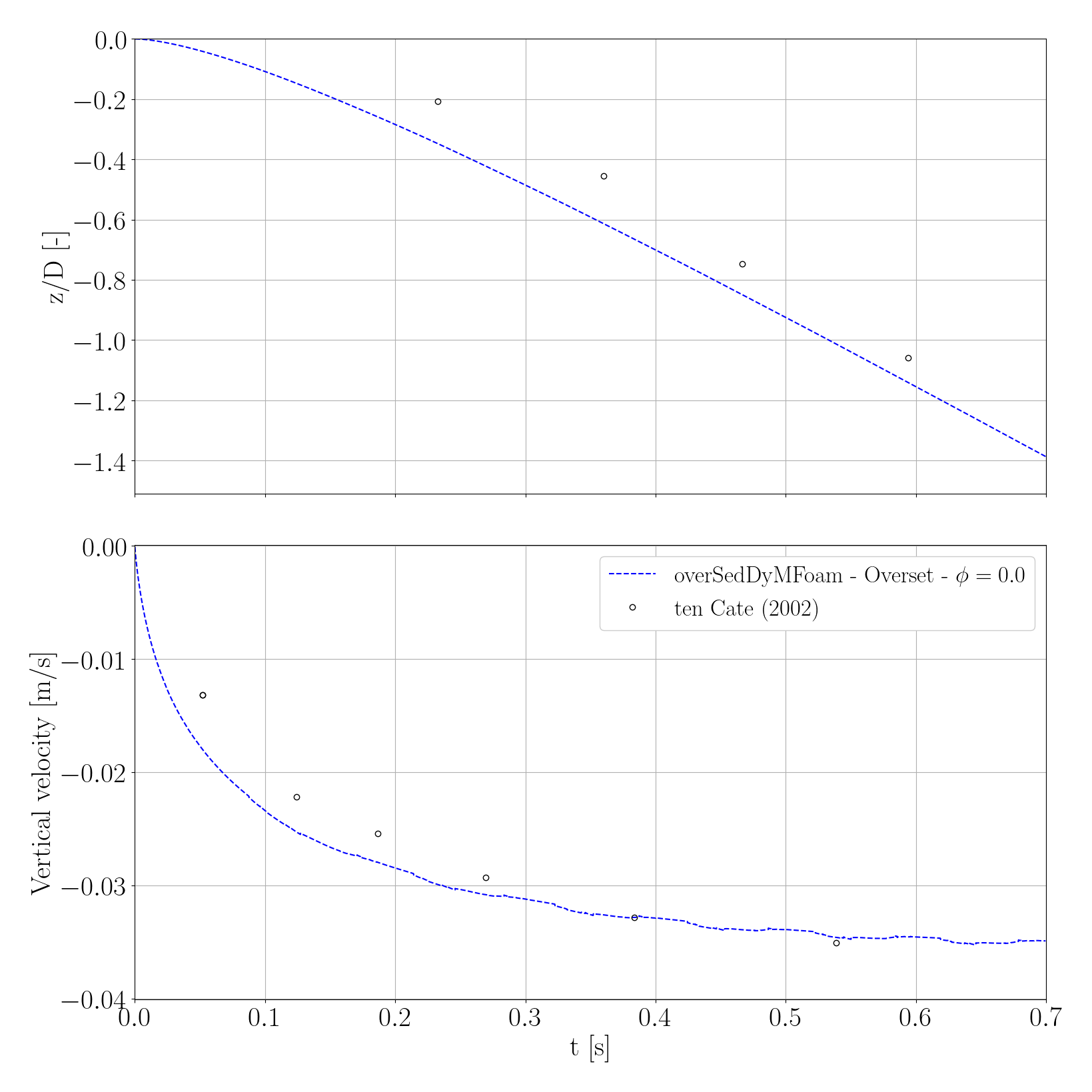
You just have to run the python script plot3DFallingSphere.py located in the folder tutorialsDyM/Py. Make sure that the chosen mesh in the script is set to DynamycMesh="Overset".
python plot3DFallingSphere.py
and you should see the following figure that shows the trajectory and velocity of the sphere falling in a pure fluid using the overset technique:
FallingSphereMorphing: Falling sphere in pure fluid using a morphing mesh
This numerical test investigates the same falling sphere presented in the previous case using a morphing mesh instead of the overset technique. The numerical case is located at tutorialsDyM/FallingSphereMorphing.
Mesh generation and setup
The numerical domain consists of a spherical mesh with a diameter of . This type of mesh can deform, but the connectivity between the cells remains unchanged. The mesh is illustrated in Figure 3.
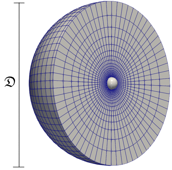
The spherical mesh is generated by running the command blockMesh in the tutorialsDyM/FallingSphereMorphing folder.
Dynamic mesh
Several mesh options and controls can be adjusted in the dynamicMeshDict dictionary located in the constant folder. For morphing meshes, the dynamicMotionSolverFvMesh solver is employed to modify the mesh topology around a rigid object. The mesh region around the rigid body is divided into three parts: the region where the mesh moves with the rigid body, the mesh morphing region, and the outer region that remains static.
Several mesh options and controls can be adjusted in the dynamicMeshDict dictionary located in the constant folder. For morphing meshes, dynamicMotionSolverFvMesh solver is employed to modify the mesh topology around a rigid object. The mesh region around the rigid body is divided into three parts: the region where the mesh moves with the rigid body, the mesh morphing region and the outer region that remains static. The part inside the innerDistance is completely body motion so it does not deform, and the region between the innerDistance and outerDistance corresponds to the mesh morphing region.
/*--------------------------------*- C++ -*----------------------------------*\
| =========                 |                                                 |
| \\      /  F ield         | OpenFOAM: The Open Source CFD Toolbox           |
|  \\    /   O peration     | Version:  v2306                                 |
|   \\  /    A nd           | Website:  www.openfoam.com                      |
|    \\/     M anipulation  |                                                 |
\*---------------------------------------------------------------------------*/
FoamFile
{
    version     2.0;
    format      ascii;
    class       dictionary;
    object      motionProperties;
}
// * * * * * * * * * * * * * * * * * * * * * * * * * * * * * * * * * * * * * //


dynamicFvMesh       dynamicMotionSolverFvMesh;

motionSolverLibs    (sixDoFRigidBodyMotionSedFoam);

motionSolver        sixDoFRigidBodyMotion;


sixDoFRigidBodyMotionCoeffs
{

    patches         (sphere);
    innerDistance   0.005;
    outerDistance   0.049;

    accelerationRelaxation 0.4;
    accelerationDamping 0.4;

    //  mass reduced by Buoyancy: (rhosolid - rhofluid ) * VolumeSphere
    mass            2.6507E-04; //volumeSphere = 1.76714e-6
    centreOfMass    ( 0 0 0 );
    momentOfInertia ( 4.45E-08 4.45E-08 4.45E-08);
    rho             rhoInf;
    rhoInf          970;
    g               (0 0 -9.81);
    report          on;
    reportToFile    on;

    solver
    {
        type Newmark;
    }

    constraints
    {

    }

}
// ************************************************************************* //
Computation launching
The simulations will run in parallel on 10 cores by executing the following commands at tutorialsDyM/FallingSphereMorphing folder:
decomposePar
mpirun -np 10 overSedDymFoam_rbgh -parallel > log.out&
One can skip all the previous steps and simply run the command *./Allrun* in the tutorialsDyM/FallingSphereMorphing folder to launch the numerical case.
Post-processing using python
You just have to run the python script plot3DFallingSphere.py located in the folder tutorialsDyM/Py. Make sure that the chosen mesh in the script is set to DynamycMesh="Morphing".
python plot3DFallingSphere.py
and you should see the following figure that shows the trajectory and velocity of the sphere falling in a pure fluid using the morphing mesh:
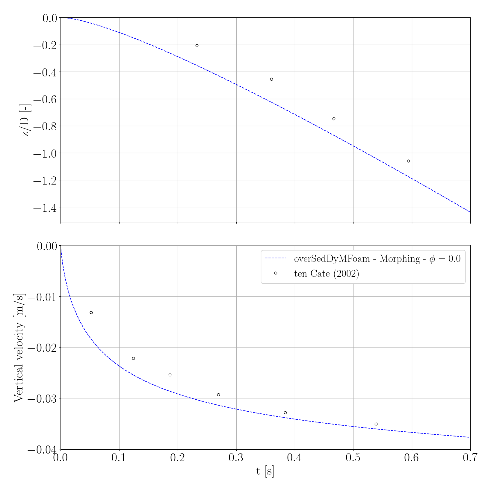
Falling sphere in a sediment suspension
In this scenario, we aim to extend the results by numerically reproducing the falling sphere in a fluid with the presence of sediments in suspension. For this numerical setup, the sediment content is set to 5 , and the particles are neutrally buoyant (i.e. same density as the fluid) with a mean diameter of . The numerical cases are located at tutorialsDyM/FallingSphereSuspensionMorphing and tutorialsDyM/FallingSphereSuspensionOverset. These two cases are just an extension of previous cases, therefore, a few modifications are required to handle the particulate phase.
Physical properties
In the constant/transportProperties file, the physical properties of the solid and fluid phases are set, such as density, kinematic viscosity and particle diameter:
/*--------------------------------*- C++ -*----------------------------------*\
| =========                 |                                                 |
| \\      /  F ield         | OpenFOAM: The Open Source CFD Toolbox           |
|  \\    /   O peration     | Version:  v2306                                 |
|   \\  /    A nd           | Website:  www.openfoam.com                      |
|    \\/     M anipulation  |                                                 |
\*---------------------------------------------------------------------------*/
FoamFile
{
    version     2.0;
    format      ascii;
    class       dictionary;
    location    "constant";
    object      transportProperties;
}
// * * * * * * * * * * * * sediment properties * * * * * * * * * * * * //
phasea
{
    rho             rho [ 1 -3 0 0 0 ] 970.01;
    nu              nu [ 0 2 -1 0 0 ] 1e-6;
    d               d [ 0 1 0 0 0 0 0 ] 290e-6;
    hExp            hExp [ 0 0  0 0 0 0 0 ] 3.15;  // hindrance exponent for drag: beta^(-hExp) (2.65 by default)
}
// * * * * * * * * * * * * fluid properties * * * * * * * * * * * * //
phaseb
{
    rho             rho [ 1 -3 0 0 0 ] 970;
    nu              nu [ 0 2 -1 0 0 0 0 ] 3.845e-4;
    d               d [ 0 1 0 0 0 0 0] 290e-6;
}
//*********************************************************************** //
transportModel  Newtonian;

nu              nu [ 0 2 -1 0 0 0 0 ] 3.845e-4 ;

nuMax           nuMax [0 2 -1 0 0 0 0] 1e3;      // viscosity limiter for the Frictional model (required for stability)

alphaSmall      alphaSmall [ 0 0 0 0 0 0 0 ] 1e-6;  // minimum volume fraction (phase a) for division by alpha

// ************************************************************************* //
The Gidaspow-Schiller-Naumann drag model, frequently employed for sediment suspensions is considered and set in constant/interfacialProperties.
/*--------------------------------*- C++ -*----------------------------------*\
| =========                 |                                                 |
| \\      /  F ield         | OpenFOAM: The Open Source CFD Toolbox           |
|  \\    /   O peration     | Version:  v2306                                 |
|   \\  /    A nd           | Website:  www.openfoam.com                      |
|    \\/     M anipulation  |                                                 |
\*---------------------------------------------------------------------------*/
FoamFile
{
    version     2.0;
    format      ascii;
    class       dictionary;
    location    "constant";
    object      interfacialProperties;
}
// * * * * * * * * * * * * * * * * * * * * * * * * * * * * * * * * * * * * * //

dragModela      GidaspowSchillerNaumann;

dragModelb      GidaspowSchillerNaumann;

dragPhase       a;


// ************************************************************************* //
Finally, the concentration of sediments can be adjusted in 0_org/alpha.a simply setting the desired volume fraction as a uniform internal field:
/*--------------------------------*- C++ -*----------------------------------*\
| =========                 |                                                 |
| \\      /  F ield         | OpenFOAM: The Open Source CFD Toolbox           |
|  \\    /   O peration     | Version:  v2306                                 |
|   \\  /    A nd           | Website:  www.openfoam.com                      |
|    \\/     M anipulation  |                                                 |
\*---------------------------------------------------------------------------*/
FoamFile
{
    version     2.0;
    format      ascii;
    class       volScalarField;
    location    "0";
    object      alpha.a;
}
// * * * * * * * * * * * * * * * * * * * * * * * * * * * * * * * * * * * * * //

dimensions      [0 0 0 0 0 0 0];

internalField   uniform 0.05;
Computation launching
The simulations of a falling sphere in a particle suspension, both using overset and morphing mesh, will run in parallel executing the same commands as in the pure fluid.
Post-processing using python
You just have to run the python script plot3DFallingSphere_suspension.py located in the folder tutorialsDyM/Py. Make sure that you select the desired mesh in the first lines of the script (DynamycMesh="Morphing" or DynamycMesh="Overset").
python plot3DFallingSphere_suspension.py
and you should see the following figure that shows the trajectory and velocity of the sphere falling in a sediment suspension:
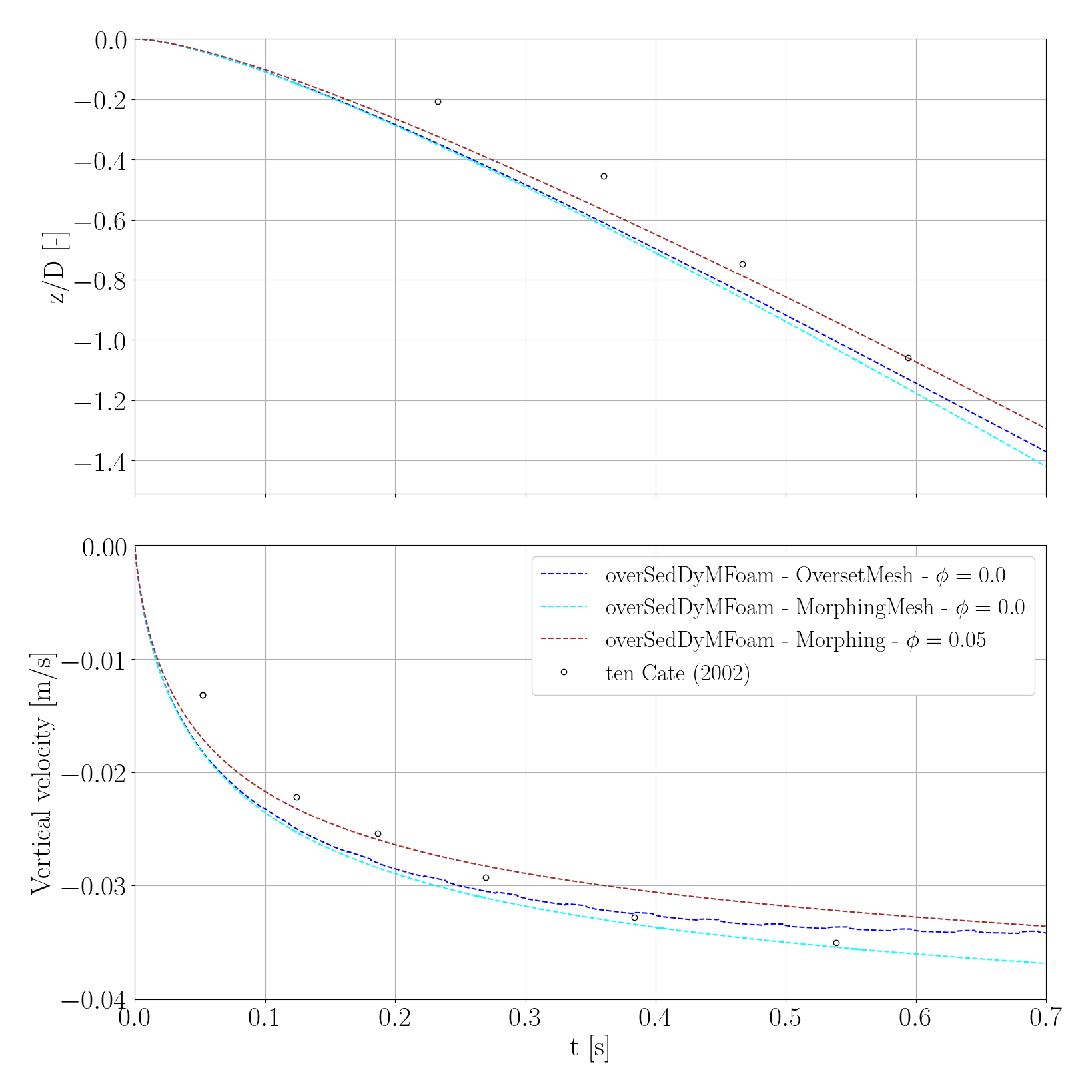
Sphere falling into a dense granular bed
This section tests the ability of sedFoam to capture the particle pressure and frictional stresses on a rigid body.
Mesh generation and setup
The computational domain is assumed to be a spherical domain with a diameter of . As shown in Figure 6, a horizontal sediment bed is included in the numerical simulation. The numerical case is located at tutorialsDyM/RestingSphereMorphing . The bed interface is located at a distance of from the lowest point of the sphere. The rest of the physical and geometrical parameters are summarized in the following table:
| Properties | Value |
|---|---|
| Sphere density | |
| Fluid density | |
| Fluid viscosity | |
| Sediment density | |
| Sediment diameter | |
| Sphere diameter |
The spherical mesh is generated by running the command blockMesh in the tutorialsDyM/RestingSphereMorphing folder.
Physical properties
In the constant/transportProperties file, the physical properties of the solid and fluid phases are set, such as density, kinematic viscosity and particle diameter:
/*--------------------------------*- C++ -*----------------------------------*\
| =========                 |                                                 |
| \\      /  F ield         | OpenFOAM: The Open Source CFD Toolbox           |
|  \\    /   O peration     | Version:  v2306                                 |
|   \\  /    A nd           | Website:  www.openfoam.com                      |
|    \\/     M anipulation  |                                                 |
\*---------------------------------------------------------------------------*/
FoamFile
{
    version     2.0;
    format      ascii;
    class       dictionary;
    location    "constant";
    object      transportProperties;
}
// * * * * * * * * * * * * sediment properties * * * * * * * * * * * * //
phasea
{
    rho         rho [ 1 -3 0 0 0 ] 2650;
    nu          nu [ 0 2 -1 0 0 ] 1.e-6;
    d           d [ 0 1 0 0 0 0 0 ] 1.e-2;
    sF              sF   [ 0 0  0 0 0 0 0 ] 1.;    // shape Factor to adjust settling velocity for non-spherical particles
    hExp        hExp [ 0 0  0 0 0 0 0 ] 2.65; // hindrance exponent for drag:
                          // beta^(-hExp) (2.65 by default)
}
// * * * * * * * * * * * * fluid properties * * * * * * * * * * * * //
phaseb
{
    rho         rho [ 1 -3 0 0 0 ] 1000;
    nu          nu [ 0 2 -1 0 0 ] 1.e-06;
    d           d [ 0 1 0 0 0 0 0 ] 1.e-2;
}
//*********************************************************************** //
transportModel  Newtonian;

nu              nu [ 0 2 -1 0 0 0 0 ] 1e-6;

// Diffusivity for mass conservation resolution (avoid num instab around shocks)
alphaDiffusion  alphaDiffusion [0 2 -1 0 0 0 0] 1e-8;

// viscosity limiter for the Frictional model (required for stability)
nuMax           nuMax [0 2 -1 0 0 0 0] 100;

// minimum volume fraction (phase a) for division by alpha
alphaSmall      alphaSmall [ 0 0 0 0 0 0 0 ] 1e-3;

// ************************************************************************* //
Because we are dealing with a dense granular material, the Ergun drag formulation is adopted to model the permeability. The drag model is set in constant/interfacialProperties as:
/*--------------------------------*- C++ -*----------------------------------*\
| =========                 |                                                 |
| \\      /  F ield         | OpenFOAM: The Open Source CFD Toolbox           |
|  \\    /   O peration     | Version:  v2306                                 |
|   \\  /    A nd           | Website:  www.openfoam.com                      |
|    \\/     M anipulation  |                                                 |
\*---------------------------------------------------------------------------*/
FoamFile
{
    version     2.0;
    format      ascii;
    class       dictionary;
    location    "constant";
    object      interfacialProperties;
}
// * * * * * * * * * * * * * * * * * * * * * * * * * * * * * * * * * * * * * //

dragModela      Ergun;

dragModelb      Ergun;

dragPhase       a;


// ************************************************************************* //
After creating the initial tome folder (execute cp -r 0_org 0), the dense sediment bed beneath the spherical object needs to be put in place. To do so, first, we need to run the initial_1D_profile/1DSedim case to get the sedimentation of the granular material. Then, mapFields utility maps the fields (including the concentration field – alpha.a) from the 1DSedim onto the corresponding fields for the 3D spherical geometry:
mapFields -sourceTime 5 initial_1D_profile/1DSedim/
Computation launching
The simulations will run in parallel on 10 cores by executing the following commands at tutorialsDyM/RestingSphereMorphing folder:
decomposePar
mpirun -np 10 overSedDymFoam_rbgh -parallel > log.out&
One can skip all the previous steps and simply run the command *./Allrun* in the tutorialsDyM/RestingSphereMorphing folder to launch the numerical case.
Post-processing using python
You just have to run the python script plotRestingSphere.py located in the folder tutorialsDyM/Py.
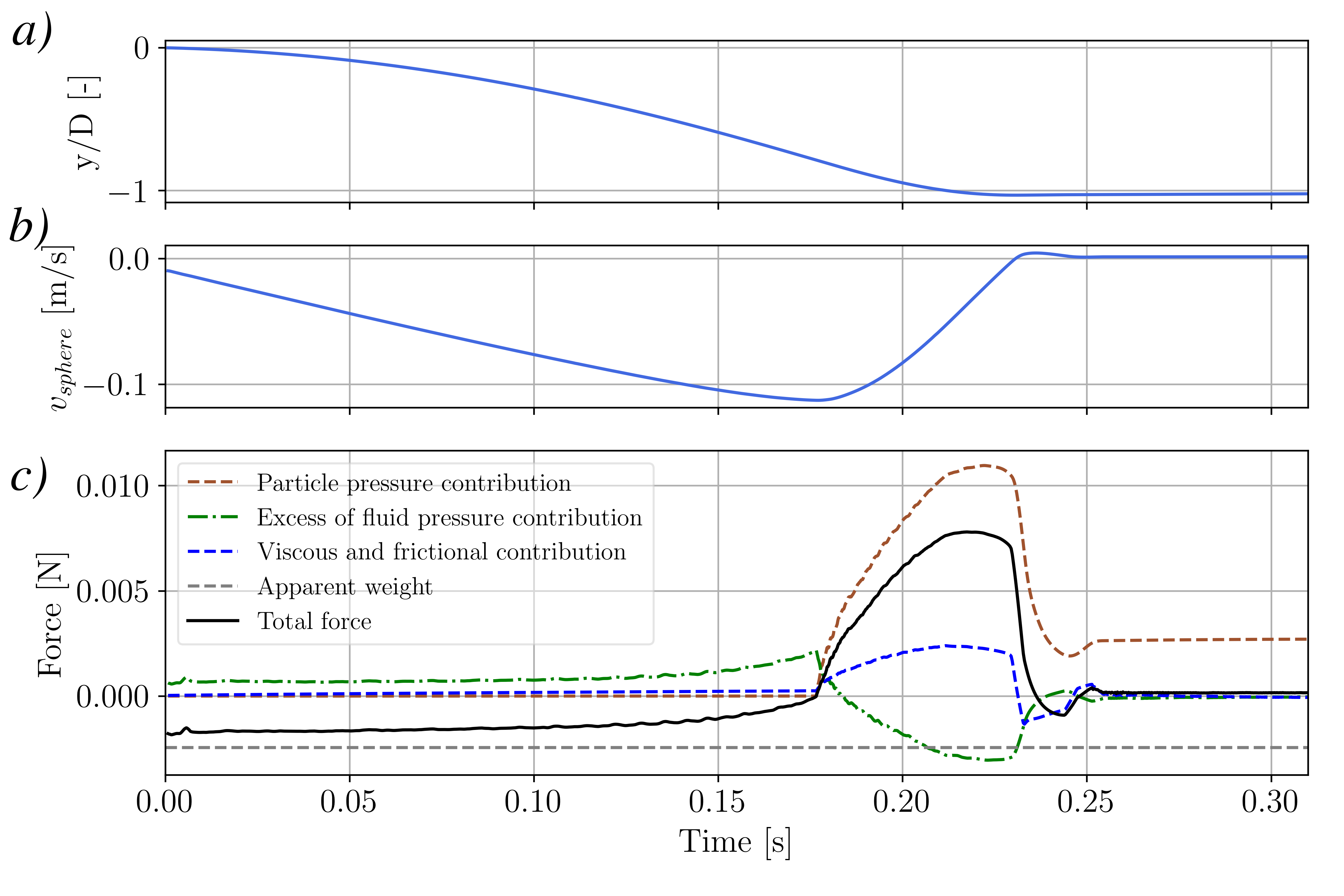
python plotRestingSphere.py
and you should see the following figure that show the trajectory and velocity of the sphere falling on a dense granular horizontal bed:
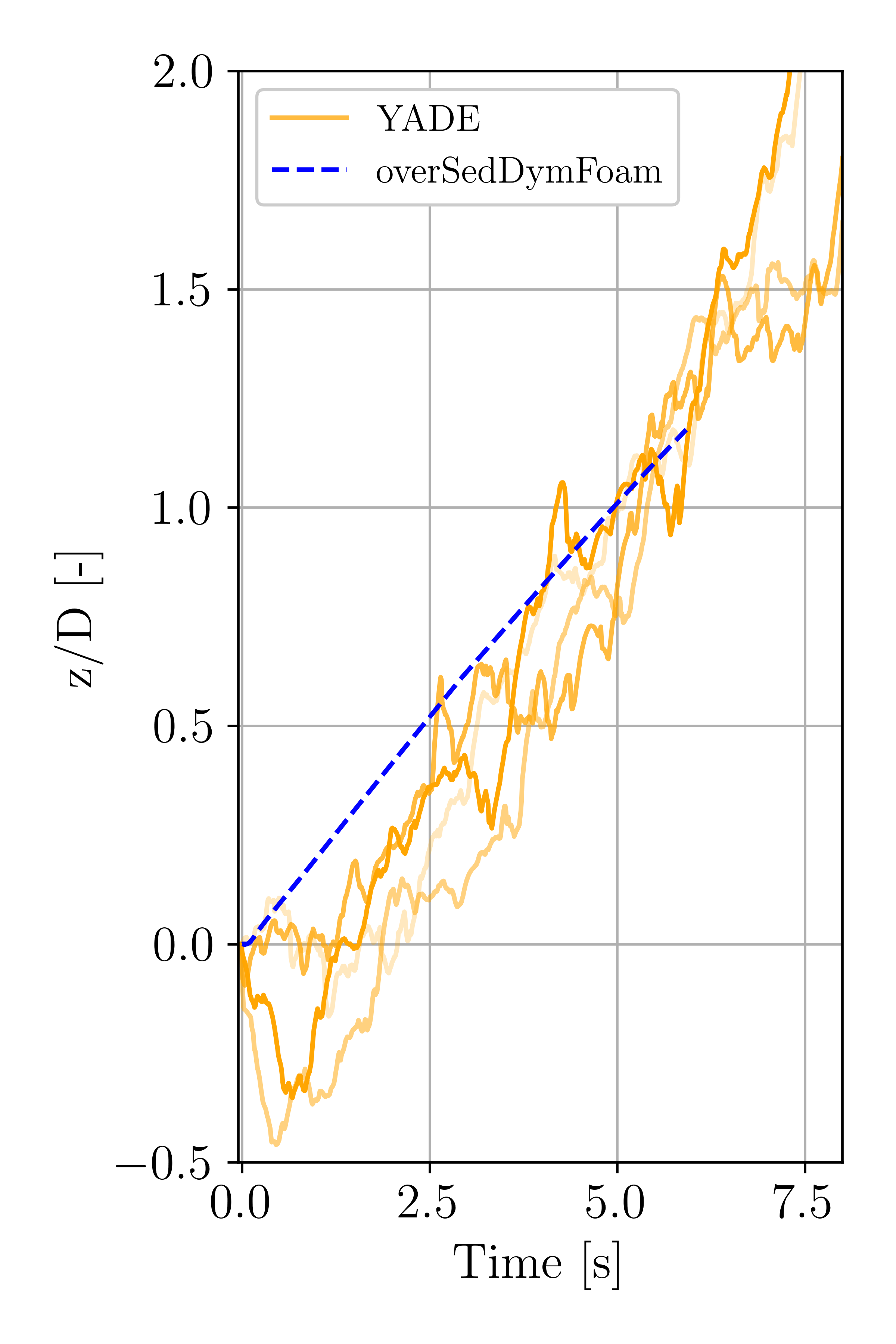
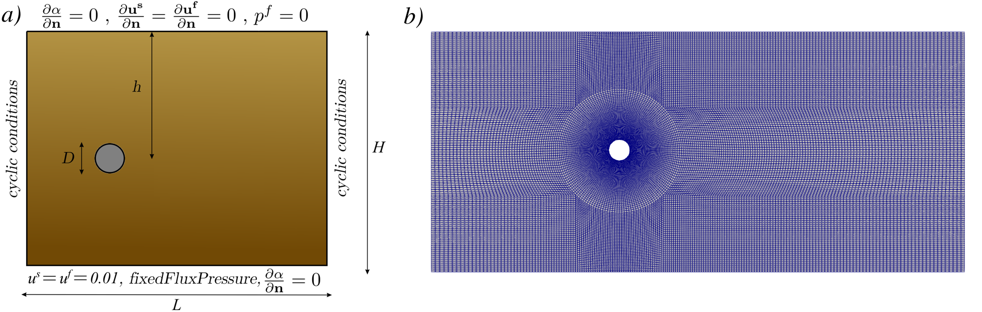
2DCylinderUniformGranularFlow: Uniform granular flow around a cylinder
In this subsection we analyze the stresses and the trajectory of an intruder immersed in a uniform granular flow. To reduce the computational cost, we use a cylinder (a 2D object in OpenFOAM) instead of the spherical intruder employed in previous numerical cases. Our approach is inspired by the work of Guillard , where lift and drag forces on a cylinder were measured under a granular flow. We adopt a similar setup, as depicted in Figure 8. More specifically, a granular packing is considered, then, the bottom plate is set to a prescribed constant velocity that induces a uniform granular flow above the bottom plate. Placing a cylinder in the granular medium distorts the flow patterns. As illustrated in Figure 8, a constant horizontal velocity of is prescribed at the bottom to generate the uniform granular flow. The initial velocity field is set to as well. DEM simulations performed using the open-source code YADE are also presented to test the accuracy of sedFoam. The employed parameters are summarized in the following table:
| Properties | Value |
|---|---|
| Intruder density | |
| Fluid density | |
| Fluid viscosity | |
| Sediment density | |
| Sediment diameter | m |
| Intruder diameter | m |
| Domain length | m |
| Domain depth | m |
| Intruder depth | m |
Mesh generation and setup
The rectangular mesh is generated by running the command blockMesh in the tutorialsDyM/2DCylinderUniformGranularFlow folder.
Physical properties
In the constant/transportProperties file, the physical properties of the solid and fluid phases are set, such as density, kinematic viscosity and particle diameter. It is worth noting that DEM simulations assume a dry granular material, however, the density ratio using sedFoam is slightly different to avoid numerical errors:
/*--------------------------------*- C++ -*----------------------------------*\
| =========                 |                                                 |
| \\      /  F ield         | OpenFOAM: The Open Source CFD Toolbox           |
|  \\    /   O peration     | Version:  v2306                                 |
|   \\  /    A nd           | Website:  www.openfoam.com                      |
|    \\/     M anipulation  |                                                 |
\*---------------------------------------------------------------------------*/
FoamFile
{
    version     2.0;
    format      ascii;
    class       dictionary;
    location    "constant";
    object      transportProperties;
}
// * * * * * * * * * * * * sediment properties * * * * * * * * * * * * //
phasea
{
    rho             rho [ 1 -3 0 0 0 ] 2500;
    nu              nu [ 0 2 -1 0 0 ] 1e-6;
    d               d [ 0 1 0 0 0 0 0 ] 0.0015;
}

phaseb
{
    rho             rho [ 1 -3 0 0 0 ] 50.;
    nu              nu [ 0 2 -1 0 0 ] 1.5e-05;
    d               d [ 0 1 0 0 0 0 0 ] 2.e-3;
}
//*********************************************************************** //
transportModel  Newtonian;

nu              nu [ 0 2 -1 0 0 0 0 ] 1.5e-05;

// Diffusivity for mass conservation resolution (avoid num instab around shocks)
alphaDiffusion  alphaDiffusion [0 2 -1 0 0 0 0] 0e-8;

nuMax           nuMax [0 2 -1 0 0 0 0] 1e1;      // viscosity limiter for the Frictional model (required for stability)

alphaSmall      alphaSmall [ 0 0 0 0 0 0 0 ] 1e-5;  // minimum volume fraction (phase a) for division by alpha

// ************************************************************************* //
Because we are dealing with a dense granular material, the Ergun drag formulation is adopted to model the permeability. The drag model is set in constant/interfacialProperties as:
/*--------------------------------*- C++ -*----------------------------------*\
| =========                 |                                                 |
| \\      /  F ield         | OpenFOAM: The Open Source CFD Toolbox           |
|  \\    /   O peration     | Version:  v2306                                 |
|   \\  /    A nd           | Website:  www.openfoam.com                      |
|    \\/     M anipulation  |                                                 |
\*---------------------------------------------------------------------------*/
FoamFile
{
    version     2.0;
    format      ascii;
    class       dictionary;
    location    "constant";
    object      interfacialProperties;
}
// * * * * * * * * * * * * * * * * * * * * * * * * * * * * * * * * * * * * * //

dragModela      Ergun;

dragModelb      Ergun;

dragPhase       a;


// ************************************************************************* //
After creating the initial time folder (execute cp -r 0_org 0), the dense granular material is generated using the sediment concentration vertical profile of a one dimensional sedimentation. To do so, first, we need to run the Case1D case to get the sedimentation of the granular material and the correct lithostatic pressure gradient. Then, mapFields utility maps the fields (including the concentration field – alpha.a) from the Case1D case onto the corresponding fields for the 2D rectangular geometry:
mapFields -sourceTime 3 Case1D/
Computation launching
The simulations will run in parallel on 10 cores by executing the following commands at tutorialsDyM/2DCylinderUniformGranularFlow folder:
decomposePar
mpirun -np 10 overSedDymFoam_rbgh -parallel > log.out&
One can skip all the previous steps and simply run the command *./Allrun* in the tutorialsDyM/2DCylinderUniformGranularFlow folder to launch the numerical case.
Post-processing using python
You just have to run the python script plot2DCylinderPosition.py located in the folder tutorialsDyM/Py.
python plot2DCylinderPosition.py
and you should see the following figure that shows the evolution of the large intruder compared to the trajectory given by YADE simulations. As reported by Guillard, the asymmetrical granular stress field results in a lift force that brings the intruder up to the surface.