LES tutorials
In this chapter LES tutorials are presented to illustrate the full SedFoam capabilities to deal with Large Eddy Simulations as well as to provide configuration files to allow for the development of new configurations both in dimensional and dimensionless forms.
3DChannel180: Favre average TKE budget of Turbulent channel flow at Retau = 180
The Favre average turbulent kinetic energy (TKE) budget can be done during the simulation using the switch in the controlDict file inside system folder. The details are discuss in the coming sections.
Pre-processing
The tutorial is distributed with sedFoam under the folder sedFoamDirectory/tutorials/3DChanel180.
Mesh and boundary conditions
The numerical domain and boundary condition details are provided in 3DChannel560: Turbulent channel flow laden with particles. The mesh consists of elements and is stretched along the axis to enhance resolution near the walls.
To be updated
Initial conditions
The flow is driven by the pressure gradient along the axis, which is dynamically adjusted at each time step to maintain the bulk velocity . This adjustment of the bulk velocity is carried out using the OpenFOAM fvOption utility.
Physical properties
The "constant" folder contains all the physical parameters or closures required to solve the flow numerically. To set the Reynolds number , the molecular viscosity has to be set in the transportProperties file as shown below (see \ndsolution page for more details).
phasea
{
    rho             rho [ 1 -3 0 0 0 ]    1;
    nu              nu  [ 0 2 -1 0 0 ]    3.6e-4; // 1/Re_tau;
    d               d   [ 0 1 0 0 0 0 0 ] 1.95e-4;
    sF              sF   [ 0 0  0 0 0 0 0 ] 1;    // shape Factor to adjust settling velocity for non-spherical particles
    hExp            hExp [ 0 0  0 0 0 0 0 ] 2.65;  // hindrance exponent for drag: beta^(-hExp) (2.65 by default)
}
// * * * * * * * * * * * * fluid properties * * * * * * * * * * * * //
phaseb
{
    rho             rho [ 1 -3 0 0 0 ] 1;
    nu              nu [ 0 2 -1 0 0 ]  3.6e-4; // 1/Re_tau;
    d               d [ 0 1 0 0 0 0 0 ] 2e-4;
    sF              sF   [ 0 0  0 0 0 0 0 ] 1;
    hExp            hExp [ 0 0  0 0 0 0 0 ] 2.65;
}
//*********************************************************************** //
transportModel  Newtonian;

nu              nu [ 0 2 -1 0 0 0 0 ] 3.6e-4; //1/Re_tau;

nuMax           nuMax [0 2 -1 0 0 0 0] 1e2;      // viscosity limiter for the Frictional model (required for stability)

alphaSmall      alphaSmall [ 0 0 0 0 0 0 0 ] 1e-6;  // minimum volume fraction (phase a) for division by alpha

// ************************************************************************* //
Running the simulation
All simulation-related parameters are specified in the controlDict file located inside the system folder. The switch for Favre-averaged turbulent kinetic energy is also found in the controlDict file. To enable Favre averaging, add the following line to the controlDict file as described in Section 3DChannel560: Turbulent channel flow laden with particles. It is recommended to start by running a warm-up simulation for approximately 100 without averaging.
You can run the sedFoam code in parallel mode. To setup the simulation, you can execute Allrun for mesh generation and turbulence initialization. Then you can run the simulation on 16 processors (default set up here) by typing:
# Run sedFoam in parallel
mpirun -np 16 sedFoam_rbgh -parallel > log&
After completing the simulation in parallel, it is necessary to reconstruct the files obtained from each processor. To do this, first, load the OpenFOAM module and execute the following command in the terminal or include it in a bash script.
reconstructPar -time 100
Control
Once the first simulation is finished, rerun the code for another 100 by turning on the averaging by setting both keywords AverageMode and favreAverage_fluid to true. You also have to modify the startTime keywork in system/controlDict to 100 and the keyword endTime to 200.
AverageMode   true;  // To enable Favre average mode keep it true or otherwise keep it false

StartAverageTime 0.0;  // Time from where you want to start averaging

favreAverage_fluid  true;   // To save the Favre average files
Post-processing
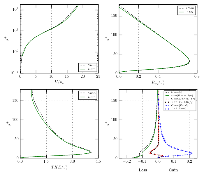
Once the simulation is completed, use the plot_tuto3DChannel180.py script located in the folder tutorial/Py/ to compare the data from sedFoam with a reference LES with a using sedFOAM and Direct Numerical Simulation (DNS) data (R. D. Moser, J. Kim & N. N. Mansour, (1998)).
3DChannel560: Turbulent channel flow laden with particles
In this tutorial, the particle-laden closed channel flow experimental configuration from Kiger and Pan (2002) is reproduced using Large-Eddy Simulation (LES).
Pre-processing
This tutorial is distributed with SedFoam under the folder sedFoamDirectory/tutorials/3DChannel560.
Mesh and boundary conditions
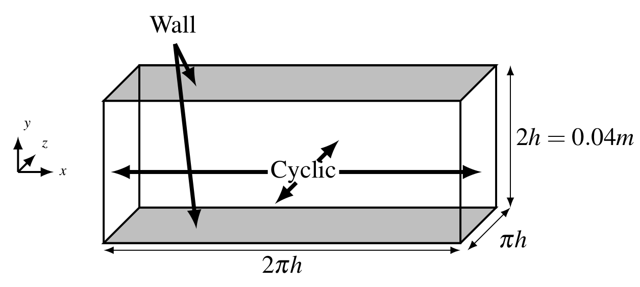
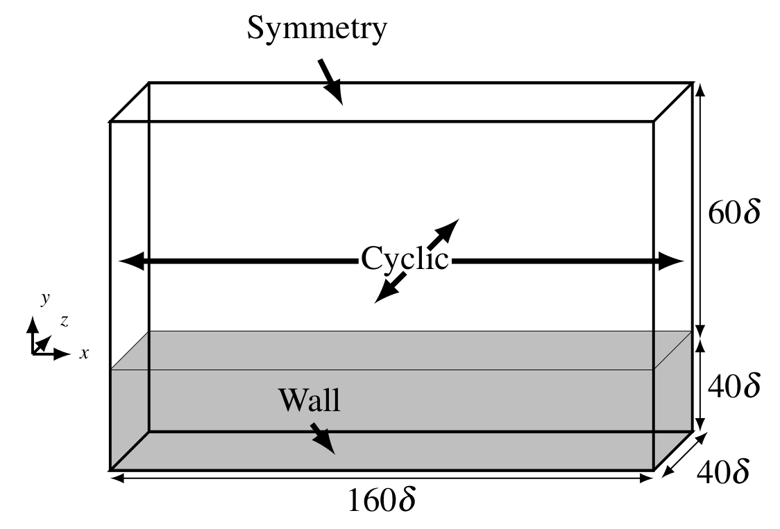
The numerical domain dimensions presented in figure 1. The numerical domain is a bi-periodic rectangular box with cyclic boundary conditions in and directions and no slip boundary condition at the top and bottom boundaries for the velocities. The gradient of any other quantities is set to zero at the walls. The mesh is composed of elements. The mesh is stretched along the -axis to increase the resolution close to the walls.
Initial conditions
The case is set up to start at time t = 0 s with a uniform concentration field and a parabolic velocity profile in the -direction with small perturbations to trigger turbulence.
The flow is driven by a pressure gradient along the -axis dynamically adjusted at each time step in order to match the experimental bulk velocity using the OpenFoam fvOption utility.
Physical properties
The transportProperties file for the 3DChannel560 case is shown below:
phasea
{
    rho             rho [ 1 -3 0 0 0 ] 2600;
    nu              nu [ 0 2 -1 0 0 ] 1e-6;
    d               d [ 0 1 0 0 0 0 0 ] 1.95e-4;
    sF              sF   [ 0 0  0 0 0 0 0 ] 1;    // shape Factor to adjust settling velocity for non-spherical particles
    hExp            hExp [ 0 0  0 0 0 0 0 ] 2.65;  // hindrance exponent for drag: beta^(-hExp) (2.65 by default)
}
// * * * * * * * * * * * * fluid properties * * * * * * * * * * * * //
phaseb
{
    rho             rho [ 1 -3 0 0 0 ] 1000;
    nu              nu [ 0 2 -1 0 0 ] 1.e-6;
    d               d [ 0 1 0 0 0 0 0 ] 2e-4;
    sF              sF   [ 0 0  0 0 0 0 0 ] 1;
    hExp            hExp [ 0 0  0 0 0 0 0 ] 2.65;
}
//*********************************************************************** //
transportModel  Newtonian;

nu              nu [ 0 2 -1 0 0 0 0 ] 1.e-6;

nuMax           nuMax [0 2 -1 0 0 0 0] 1e2;      // viscosity limiter for the Frictional model (required for stability)

alphaSmall      alphaSmall [ 0 0 0 0 0 0 0 ] 1e-3;  // minimum volume fraction (phase a) for division by alpha
The physical property of the particles (diameter and density) and of the fluid (density and kinematic viscosity) have been set to the values given in Kiger and Pan (2002).
Control
The system/controlDict file indicates that for this case, the time step is set to a constant value of s that ensure to have a maximum Courant number on the order of 0.3 for stability reasons.
The end time of the simulation is set to 8 for initial development of turbulence. After 8 seconds, the simulation should be continued by changing the end time to 16 seconds and setting the favreAveraging keyword to true to perform temporal averaging of flow variables.
application     sedFoam_rbgh;

startFrom       latestTime;

startTime       0;

stopAt          endTime;

endTime         8;
//endTime         16;

deltaT          2e-4;

writeControl    runTime;

writeInterval   0.5;

purgeWrite      0;

writeFormat     binary;

writePrecision  6;

writeCompression off;

timeFormat      general;

timePrecision   6;

runTimeModifiable true;

maxAlphaCo  1;

favreAveraging false;
Computation launching
As for the previous case, you can launch the computation by executing Allrun for turbulence initialization. The simulations is run in parallel on 16 cores. Once the end time has been modified and favreAveraging keyword set to true, you can launch the computation of time average variables by executing AllrunAverage.
Post-processing using python
The post-processing python scripts writedata_tuto3DChannel560.py and plot_tuto3DChannel560.py are located in the folder tutorials/Py. To run this script, the latest output (16s) should be reconstructed.
The script writedata_tuto3DChannel560.py reads time averaged OpenFoam data, perform a spatial averaging operation and stores the 1D vertical profiles in a netCDF file located in the postProcessing directory of the case.
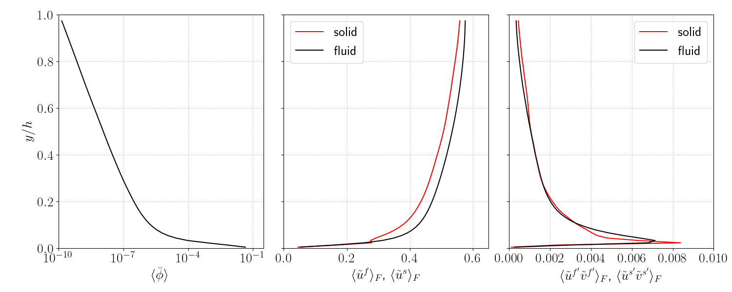
The script plot_tuto3DChannel560.py reads the netCDF file and plots vertical profile of concentration, velocities and Reynolds stresses
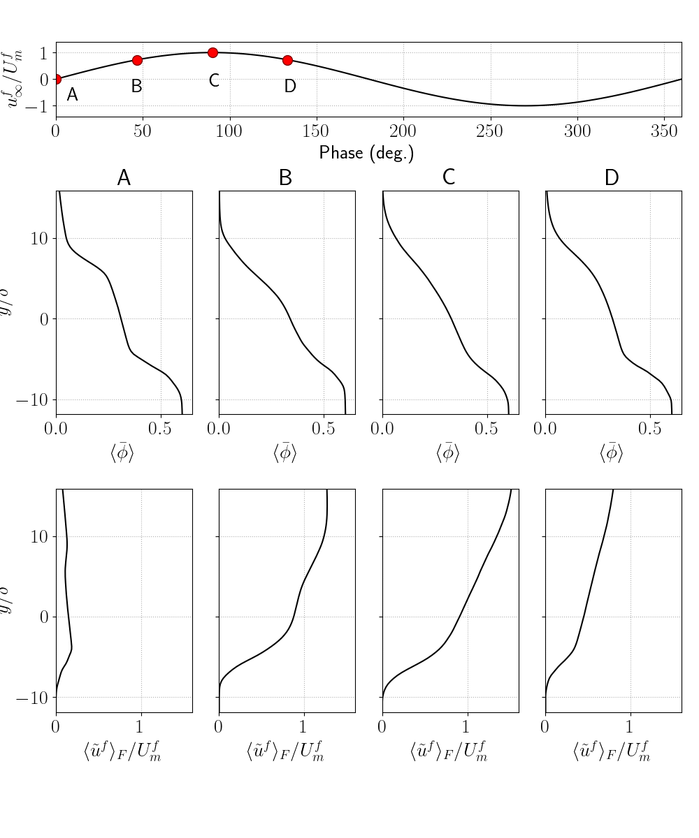
3DOscillSheetFlow: Oscillatory sheet flow
In this tutorial, the oscillatory sheet flow experimental configuration with fine sand from O'Donoghue and Wright (2004) is reproduced using Large-Eddy Simulation (LES).
Pre-processing
This tutorial is distributed with SedFoam under the folder sedFoamDirectory/tutorials/3DOscillSheetFlow.
Mesh and boundary conditions
The numerical domain is a periodic box presented in figure 3 with and the wave angular frequency. The mesh is composed of elements with celles refined at the location of the deposited sediment bed. A symmetry boundary condition is applied at the top boundary, a smooth wall boundary condition is applied at the bottom boundary and cyclic boundary conditions are applied for the lateral boundaries.
Initial conditions
The case is set up to start at time t = 0 s.
The flow is driven by a sinusoidal pressure gradient defined in constant/forceProperties along the -axis to match the experimental freestream velocity
Physical properties
The transportProperties file for the 3DOscillSheetFlow case is shown below:
phasea
{
    rho             rho [ 1 -3 0 0 0 ] 2650;
    nu              nu [ 0 2 -1 0 0 ] 1e-6;
    d               d [ 0 1 0 0 0 0 0 ] 1.5e-4;
    sF              sF   [ 0 0  0 0 0 0 0 ] 1;    // shape Factor to adjust settling velocity for non-spherical particles
    hExp            hExp [ 0 0  0 0 0 0 0 ] 2.65;  // hindrance exponent for drag: beta^(-hExp) (2.65 by default)
}
// * * * * * * * * * * * * fluid properties * * * * * * * * * * * * //
phaseb
{
    rho             rho [ 1 -3 0 0 0 ] 1000;
    nu              nu [ 0 2 -1 0 0 ] 1.e-6;
    d               d [ 0 1 0 0 0 0 0 ] 1.5e-4;
    sF              sF   [ 0 0  0 0 0 0 0 ] 1;
    hExp            hExp [ 0 0  0 0 0 0 0 ] 2.65;
}
//*********************************************************************** //
transportModel  Newtonian;

nu              nu [ 0 2 -1 0 0 0 0 ] 1.e-6;

nuMax           nuMax [0 2 -1 0 0 0 0] 1e2;      // viscosity limiter for the Frictional model (required for stability)

alphaSmall      alphaSmall [ 0 0 0 0 0 0 0 ] 1e-5;  // minimum volume fraction (phase a) for division by alpha
The physical property of the particles (diameter and density) and of the fluid (density and kinematic viscosity) have been set to the values given in O'Donoghue and Wright (2004).
Control
The system/controlDict file indicates that for this case the time step is adaptative to have a maximum Courant number (maxCo) below 0.3 and that the computation ends at 40s of dynamics.
application     sedFoam_rbgh;

startFrom       latestTime;

startTime       0;

stopAt          endTime;

endTime         40;

deltaT          2e-4;

writeControl    adjustableRunTime;

writeInterval   0.25;

purgeWrite      0;

writeFormat     binary;

writePrecision  6;

writeCompression off;

timeFormat      general;

timePrecision   6;

runTimeModifiable true;

adjustTimeStep yes;

maxCo          0.3;

maxAlphaCo     0.3;

maxDeltaT      1e-3;
Computation launching
As for the previous case, you can launch the computation by executing Allrun. The simulations is run in parallel on 16 cores.
Post-processing using python
The post-processing python scripts writedata_tuto3DOscillSheetFlow.py and plot_tuto3DOscillSheetFlow.py are located in the folder tutorials/Py. To run this script, all the simulation outputs after 20s (and only them) should be reconstructed using the following command:
reconstructPar -time '20:'
The script writedata_tuto3DOscillSheetFlow.py reads OpenFoam data, performs a spatial averaging operation, then performs a phase averaging operation taking into account four wave periods and stores the 1D vertical profiles in netCDF files located in the postProcessing directory of the case.
The script plot_tuto3DOscillSheetFlow.py reads the netCDF files and plots vertical profile of concentration, velocities and Reynolds stresses at different moments of the wave period.