Laminar flow tutorials
In this chapter we shall describe in detail the process of setup, simulation and post-processing for SedFoam test cases in the laminar flow regime. All the tutorial cases are in the tutorials/laminar directory. The text herein is highly inspired from the OpenFOAM user-guide for the cavity tutorial available at http:/
The test cases provided with SedFoam are aimed to facilitate the learning as well as the development of new configurations. If you develop new feature do not hesitate to share your development with us so that we can incorporate them in the github repository and others will benefit from your work the way you benefited from the original SedFoam version!
A number of one-dimensional test cases are provided with reference solutions, analytical, experimental or numerical, to validate SedFoam implementation and developments. Most of these test cases are used in the contiunous integration procedure to verify new developments in SedFoam.
1DSedim: Pure sedimentation
This tutorial will describe how to pre-process, run and post-process a case corresponding to a pure sedimentation problem in a one-dimensional configuration using the two-phase flow equations. The geometry is shown in Figure 1 in which bottom boundary is a wall and the top boundary is an open boundary. Initially, the flow is at rest and will be solved on a uniform mesh using the SedFoam solver for laminar, isothermal, incompressible two-phase flow. The numerical results are compared with experiments to validate the model in terms of settling curves, time evolution of concentration interface, and concentration profiles.
Pre-processing
Like in OpenFOAM, cases are setup by editing case files using a text editor such as atome, vscode/vscodium, emacs, vi, gedit, nedit, etc. The I/O uses a dictionary format with keywords. A case involves data for mesh, fields, properties, control parameters, etc that are stored in a set of files within a case directory rather than in a single case file. The case directory is given a suitably descriptive name. This tutorial consists of a set of cases located in the SedFoam distribution under the folder sedFoamDirectory/turheolotorials/laminar/1DSedim.
Mesh generation
OpenFOAM always operates in a 3 dimensional Cartesian coordinate system and all geometries are generated in 3 dimensions. OpenFOAM solves the case in 3 dimensions by default but can be instructed to solve in 2 dimensions by specifying a ‘special’ empty boundary condition on boundaries normal to the (3rd) dimension for which no solution is required. In 2 dimensions, the directions x and y are always chosen even if the mesh is given in the x-z plane.
The sedimentation domain consists of a rectangle of side length L = 0.006 m in the x–y plane and of height h=0.06 m in the vertical direction z. The side length is chosen to ensure a unity cell aspect ratio. A uniform mesh of 1 by 1 by 100 cells will be used. The block structure is shown in Figure 1.
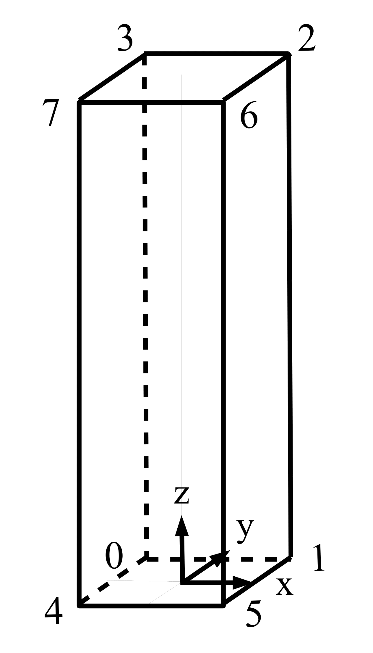
The mesh generator supplied with OpenFOAM, blockMesh, generates meshes from a description specified in an input dictionary, blockMeshDict located in the constant/polyMesh directory for a given case. The blockMeshDict entries for this case are as follows:
/*--------------------------------*- C++ -*----------------------------------*\
| =========                 |                                                 |
| \\      /  F ield         | OpenFOAM: The Open Source CFD Toolbox           |
|  \\    /   O peration     | Version:  1.7.1                                 |
|   \\  /    A nd           | Web:      www.OpenFOAM.com                      |
|    \\/     M anipulation  |                                                 |
\*---------------------------------------------------------------------------*/
FoamFile
{
    version     2.0;
    format      ascii;
    class       dictionary;
    object      blockMeshDict;
}
// * * * * * * * * * * * * * * * * * * * * * * * * * * * * * * * * * * * * * //

scale 0.06;

vertices
(
    (-0.005 0   0.005) //0
    ( 0.005 0   0.005) //1
    ( 0.005 1.  0.005) //2
    (-0.005 1.  0.005) //3
    (-0.005 0  -0.005) //4
    ( 0.005 0  -0.005) //5
    ( 0.005 1. -0.005) //6
    (-0.005 1. -0.005) //7
);

blocks
(
    hex (0 1 5 4 3 2 6 7) (1 1 200) simpleGrading (1 1 1)
);

edges
(
);

boundary
(
    inlet
    {
     type   cyclic;
     neighbourPatch outlet;
     faces ((0 3 7 4));
    }
    outlet
    {
     type   cyclic;
     neighbourPatch  inlet;
     faces  ((1 5 6 2));
    }
    top
    {
     type wall;
        faces ((7 6 2 3));
    }
    bottom
    {
     type wall;
     faces ((0 4 5 1));
    }
    frontAndBackPlanes
    {
    type empty;
    faces (
           (0 1 2 3)
           (4 7 6 5)
          );
    }
);

mergePatchPairs
(
);

// ************************************************************************* //
The file first contains header information in the form of a banner (lines 1-7), then file information contained in a FoamFile sub-dictionary, delimited by curly braces ({…}).
The file specifies coordinates of the block vertices; then, it defines the blocks (here, only 1) from the vertex labels and the number of cells within it; and finally, it defines the boundary patches. The user is encouraged to consult the official documentation here to understand the meaning of the entries in the blockMeshDict file.
The mesh is generated by running the command blockMesh. This is done simply by typing in the terminal:
blockMesh
The running status of blockMesh is reported in the terminal window. Any mistakes in the blockMeshDict file are picked up by blockMesh and the resulting error message directs the user to the line in the file where the problem occurred. There should be no error messages at this stage.
Boundary and initial conditions
Once the mesh generation is complete, the user can look at this initial fields set up for this case. The case is set up to start at time t = 0 s, so the initial field data is stored in a 0_org sub-directory of the 1DSedim directory. The 0_org sub-directory contains several files: alpha.a, U.a, U.b, p_rbgh, muI, pa, Theta, one for each of the solid phase volume fraction (alpha.a), velocities of solid and fluid phases (U.a and U.b), the reduced pressure (p_rbgh) fields whose initial values and boundary conditions must be set. Let us examine file U.a:
dimensions      [0 1 -1 0 0 0 0];

internalField   uniform (0 0 0);

boundaryField
{
    inlet
    {
        type            cyclic;
    }
    outlet
    {
        type            cyclic;
    }
    top
    {
        type            zeroGradient;
    }
    bottom
    {
        type            fixedValue;
        value           uniform (0 0 0);
    }
    frontAndBackPlanes
    {
        type            empty;
    }
}
There are 3 principal entries in field data files:
-dimensions: specifies the dimensions of the field, here velocity, i.e. m s ;
-internalField: the internal field data which are set to be uniform;
-boundaryField: the boundary field data that includes boundary conditions and data for all the boundary patches.
For this case, boundary conditions consist of cyclic boundaries at the inlet and outlet (left and right boundaries) and walls at the top and bottom boundaries, the top boundary is zeroGradient whereas the bottom boundary is a no-slip boundary conditions i.e zero velocity at the wall. The frontAndBack patch represents the front and back planes of the 2D case and therefore must be set as empty.
The user can, similarly, examine the fluid phase velocity field in the 0_org/U.b file. The solid phase volume fraction has zeroGradient boundary conditions at the top and bottom boundaries whereas the pressure has fixedValue at the top boundary (equivalent to setting the atmospheric pressure) and a fixedFluxPressure at the bottom boundary. We shall explain below what this boundary condition means.
Physical properties
The physical properties for the case are stored in dictionaries whose names are given the suffix …Properties, located in the Dictionaries directory tree. For a SedFoam case, there are 8 property files: transportProperties, interfacialProperties, ppProperties, granularRheologyProperties, kineticTheoryProperties, RASProperties twophaseRASProperties
In the transport property file, the physical properties of the solid and fluid phases are set, such as density, kinematic viscosity and particle diameter.
// * * * * * * * * * * * * sediment properties * * * * * * * * * * * * //
phasea
{
    rho             rho [ 1 -3 0 0 0 ] 1050;
    nu              nu [ 0 2 -1 0 0 ] 1e-6;
    d               d [ 0 1 0 0 0 0 0 ] 290e-6;
    hExp            hExp [ 0 0  0 0 0 0 0 ] 3.15;  // hindrance exponent for drag: beta^(-hExp) (2.65 by default)
}
// * * * * * * * * * * * * fluid properties * * * * * * * * * * * * //
phaseb
{
    rho             rho [ 1 -3 0 0 0 ] 950;
    nu              nu [ 0 2 -1 0 0 ] 2.105e-05;
    d               d [ 0 1 0 0 0 0 0 ] 290e-6;
}
//*********************************************************************** //
transportModel  Newtonian;

nu              nu [ 0 2 -1 0 0 0 0 ] 2.105e-05;

nuMax           nuMax [0 2 -1 0 0 0 0] 1e0;      // viscosity limiter for the Frictional model (required for stability)

alphaSmall      alphaSmall [ 0 0 0 0 0 0 0 ] 1e-6;  // minimum volume fraction (phase a) for division by alpha
The hindrance function exponent of the Richardson-Zaki law can be tuned using the parameter hExp. This is important for this first test case which is in the laminar regime for the drag. The transportModel has to be prescribed when using turbulence model, it is present here for compatibility with the other test cases. The nuMax value is a viscosity limiter for the all the viscosities, it allows the user to control the numerical stability of the solver and will be discussed in the second test case. It is especially important as some shear stress terms are discretized explicitly and the frictional viscosity can reach huge values. The alphaSmall value is used to regularise the division by alpha.a in the source code, the default value is set to .
The dictionary interfacialProperties allows to specify the drag model:
dragModela      GidaspowSchillerNaumann;

dragModelb      GidaspowSchillerNaumann;

dragPhase       a;
The model chosen here is GidaspowSchilerNaumann that corresponds to the drag force around a spherical particle corrected by a hindrance function ( ).
The dictionary ppProperties contains the information concerning the permanent contact contribution to the solid phase pressure. In SedFoam, the model of Johnson and Jackson (1987) is used:
ppModel          JohnsonJackson;

alphaMax         alphaMax [ 0 0 0 0 0 0 0 ] 0.635;

alphaMinFriction alphaMinFriction [ 0 0 0 0 0 0 0 ] 0.57;

Fr               Fr [ 1 -1 -2 0 0 0 0 ] 5e-2;

eta0             eta0 [ 0 0 0 0 0 0 0 ] 3;

eta1             eta1 [ 0 0 0 0 0 0 0 ] 5;

packingLimiter  no;
And the dictionary granularRheologyProperties controls the granular rheology part:
granularRheology   on;

granularDilatancy  off;

granularCohesion off;

alphaMaxG       alphaMaxG [ 0 0 0 0 0 0 0 ] 0.6;

mus             mus  [ 0 0 0 0 0 0 0 ] 0.24;

mu2             mu2  [ 0 0 0 0 0 0 0 ] 0.39;

I0              I0  [ 0 0 0 0 0 0 0 ] 0.01;

Bphi            Bphi [ 0 0 0 0 0 0 0 ] 1.;

n               n [ 0 0 0 0 0 0 0 ] 1.;

Dsmall          Dsmall [ 0 0 -1 0 0 0 0 ] 1e-4;

relaxPa         relaxPa [ 0 0 0 0 0 0 0 ] 1;

FrictionModel   Coulomb;

PPressureModel  none;

FluidViscosityModel Einstein;
On the first line the switch granularRheology allows to turn on and off this module. The keywords FrictionModel, PPressureModel and FluidViscosityModel allow to choose the friction model, the shear induced particle pressure model and the effective viscosity model (see Input Parameters for details).
For the present case the granularRheology is set to Coulomb and the FluidViscosityModel is used for the effective viscosity model and an Einstein model is used. All the details concerning the different models can be found in the Geophysical Model Development paper on SedFoam.
The remaining dictionaries are not used for this tutorial and will not be detailed here. Their content will be explained in the next tutorials when they are used.
Control
Input data related to the control of time and reading and writing of the solution data are read from the controlDict dictionary. The user should view this file as a case control file, it is located in the system directory.
The start/stop times and the time step for the run must be set. In this tutorial we wish to start the run at time t = 0 which means that OpenFOAM needs to read field data from a directory named 0. Therefore we set the startFrom keyword to startTime and then specify the startTime keyword to be 0.
As the simulation progresses we wish to write results at certain intervals of time that we can later view with a post-processing package. The writeControl keyword presents several options for setting the time at which the results are written; here we select the adjustableRunTime option which specifies that results are written every writeInterval seconds of simulated time, adjusting the time steps to coincide with the writeInterval if necessary and the time step is automatically adjusted using adjustTimeStep = on. The time step controlled using different criteria on Courant numbers based on the maximum velocity, the relative velocity ( ) and the interfacial Courant number. The maximum values of the Courant numbers (maxCo and maxAlphaCo) are set in the controlDict and the maximum value of the time step is controlled by the parameter maxDeltaT.
OpenFOAM creates a new directory named after the current time, e.g. 20 s, on each occasion that it writes a set of data. For this case, the entries in the controlDict are shown below:
application     sedFoam;

startFrom       latestTime;

startTime       0;

stopAt          endTime;

endTime         1800;

deltaT          1e-5;

writeControl    adjustableRunTime;

writeInterval   20;

purgeWrite      0;

writeFormat     ascii;

writePrecision  6;

timeFormat      general;

timePrecision   6;

runTimeModifiable on;

adjustTimeStep  on;

maxCo           0.3;

maxAlphaCo      0.3;

maxDeltaT       2e-1;
Discretisation and linear-solver settings
The numerical schemes and linear solvers are set in the system/fvSchemes and system/fvSolution files respectively.
Concerning the numerical schemes, the time discretisation is an Euler implicit scheme, the divergence terms are of Gauss limitedLinear type (2nd order centered schemes with a Sweby limiter) and the laplacian scheme is Gauss linear corrected for all terms. The fvScheme file is shown below:
ddtSchemes
{
    default         Euler implicit;
}

gradSchemes
{
        default         Gauss linear;
}

divSchemes
{
    default         none;
// alphaEqn
    div(phi,alpha)  Gauss upwind;//limitedLinear01 1;
    div(phir,alpha) Gauss upwind;//limitedLinear01 1;
// UEqn
    div(phi.a,U.a)    Gauss limitedLinearV 1;
    div(phi.b,U.b)    Gauss limitedLinearV 1;
    div(phiRa,Ua)   Gauss limitedLinear 1;
    div(phiRb,Ub)   Gauss limitedLinear 1;
// pEqn
    div(alpha,nu)   Gauss linear;
// alphaPlastic
    div(phia,alphaPlastic)   Gauss limitedLinear01 1;
// pa
    div(phia,pa_new_value)   Gauss limitedLinear 1;
}

laplacianSchemes
{
    default         none;
// UEqn
    laplacian(nuEffa,U.a) Gauss linear corrected;
    laplacian(nuEffb,U.b) Gauss linear corrected;
    laplacian(nuFra,U.a)  Gauss linear corrected;
// pEqn
    laplacian((rho*(1|A(U))),p_rbgh) Gauss linear corrected;
}

interpolationSchemes
{
    default  linear;
}

snGradSchemes
{
    default         corrected;
}

fluxRequired
{
    default         no;
    p_rbgh               ;
}
In the system/fvSolution file, the user can specify the linear solver he/she wants to use for each equation and the tolerance for the resolution. The user can also control the number of corrector steps and non-orthogonal correctors (useless for cartesian grids) for the PIMPLE algorithm. In the present case, a single PIMPLE corrector is enough the residual of the pressure equation is shown to converge well. The fvSolution file is reproduced below:
solvers
{
    p_rbgh
    {
        solver          GAMG;
        tolerance       1e-9;
        relTol          0.0001;
        smoother        DIC;
        nPreSweeps      0;
        nPostSweeps     2;
        nFinestSweeps   2;
        cacheAgglomeration true;
        nCellsInCoarsestLevel 10;
        agglomerator    faceAreaPair;
        mergeLevels     1;
    }

    p_rbghFinal
    {
        $p_rbgh;
        tolerance       1e-9;
        relTol          0;
    }
    "(alpha.a|U.a|U.b|pa_new_value|alphaPlastic)"
    {
        solver          PBiCG;
        preconditioner  DILU;
        tolerance       1e-9;
        relTol          0;
    }
    "(alpha.aFinal|U.aFinal|U.bFinal|paFinal|alphaPlasticFinal)"
    {
        solver          PBiCG;
        preconditioner  DILU;
        tolerance       1e-9;
        relTol          0;
    }
}

PIMPLE
{
    momentumPredictor 0;
    nOuterCorrectors  1;
    nCorrectors     1;
    nNonOrthogonalCorrectors 0;
    correctAlpha    0;
    nAlphaCorr      1;
    pRefCell        0;
    pRefValue       0;
}


relaxationFactors
{
    fields
    {
        p_rbgh               1.;
        p_rbghFinal          1;
    }
    equations
    {
        "U.a|U.b"             1.;
        "(U.a|U.b)Final"      1;
    }

}
Running sedFoam_rbgh
The easiest way to run the test case is to run the shell script:
#!/bin/sh

# Create the mesh
blockMesh

# create the intial time folder
cp -r 0_org 0

# Run sedFoam
sedFoam_rbgh > log&
The script is self documented, the blockMesh command has already been introduced. The initial condition stored in the 0_org folder is first copied to the zero (0) folder. The initial condition for solid phase volume fraction profile alpha.a is set using codeStream following an hyperbolic tangent profile described in the file 0_org/alpha.a as follows:
internalField   #codeStream
{
    codeInclude
    #{
        #include "fvCFD.H"
    #};

    codeOptions
    #{
        -I$(LIB_SRC)/finiteVolume/lnInclude \
        -I$(LIB_SRC)/meshTools/lnInclude
    #};
    codeLibs
    #{
        -lfiniteVolume \
        -lmeshTools
    #};
    code
    #{
        const IOdictionary& d = static_cast<const IOdictionary&>(dict);
        const fvMesh& mesh = refCast<const fvMesh>(d.db());
        scalarField alpha_a(mesh.nCells(), 0);

        forAll(mesh.C(), i)
        {
            scalar y = mesh.C()[i].y();
            if (y < 0.049)
            {
                alpha_a[i] = 0.5;
            }
            else
            {
                alpha_a[i] = 0.5*0.5*(1.0+tanh((y-0.054)/(0.0490-y)*10.0));
            }
        }
// OpenFoam.com version and Old OpenFoam.org (<= 6)
        alpha_a.writeEntry("", os);
// New OpenFoam.org version (>=7)
//        writeEntry(os, "", alpha_a);
    #};
The code is run using the command sedFoam_rbgh in the terminal. The "> log &" allows to run the code in batch and write the output in the file log. The run can be monitored using the command
tail -100 log
comment: Shall we replace the batch execution by an interactive run to avoid beginners to run multiple times the code without knowing how to kill the process.
Post-processing
Using paraview
The reader is referred to the OpenFOAM tutorial for the lid driven cavity for the basic manipulation on paraview such as viewing loading the data or viewing the mesh (http:/
Using fluidfoam
The postprocessing using python requires the installation of the package fluidfoam available at git clone https:/
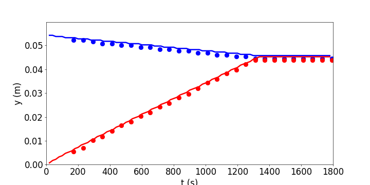
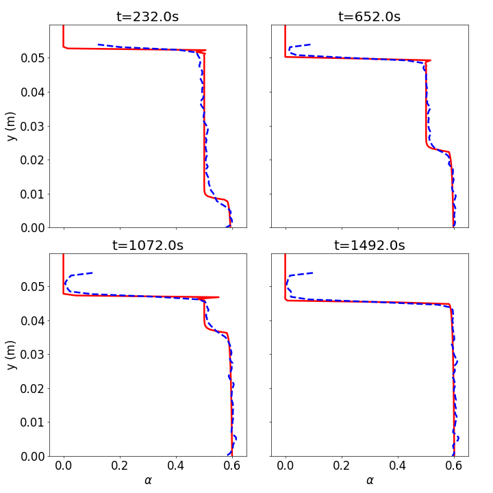
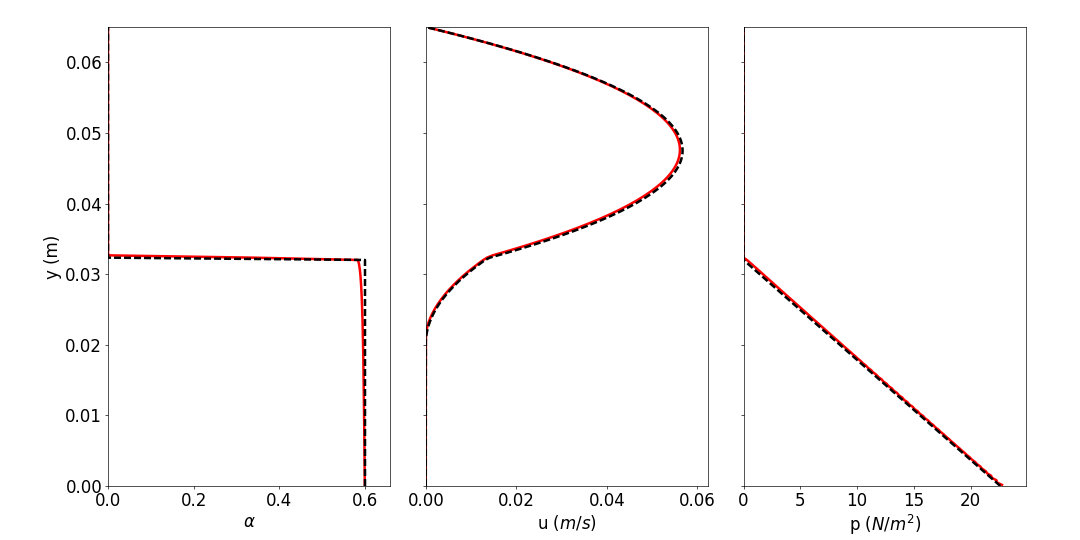
python plot_tuto1DSedim.py
and you should see the following figures:
1DBedload: Laminar bedLoad
We consider a flat particle bed submitted to a Poiseuille flow driven by a pressure gradient in a horizontal channel. This situation has been studied experimentally, analytically and numerically by Ouriemi et al. (2009) and Aussillous et al. (2013). The goal of this tutorial is to illustrate the ability of SedFoam to reproduce dense granular flows using the dense granular flow rheology . For this purpose SedFoam will be first compared with the analytical solution from Aussillous et al. (2013) using a Coulomb friction rheology. In a second part, the results obtained using the rheology are compared with a simple 1D numerical model.
Pre-processing
This tutorial is distributed with sedFoam under the folder sedFoamDirectory/tutorials/laminar/1DBedLoad.
Mesh generation
The numerical domain consists of a rectangle of side length L = 0.0065 m in the x-y plane and of height h=0.065 m in the vertical direction z. The side length is chosen to ensure a unity cell aspect ratio. A uniform mesh of 1 by 1 by 200 cells will be used. The block structure is the same as for the Sedimentation test case shown in Figure 1.
The mesh is generated by running blockMesh within the case directory:
blockMesh
Boundary and initial conditions
The case is set up to start at time t = 0 s, again the initial field data are stored in a 0_org sub-directory of the case directory. The 0_org sub-directory contains several files: alpha.a, alphaMinFriction, alphaPlastic, U.a, U.b, p_rbgh, muI, pa, pa_new, Theta, one for each of the solid phase volume fraction (alpha.a), velocities of solid and fluid phases (U.a and U.b), the reduced pressure (p_rbgh) fields whose initial values and boundary conditions must be set. Compared with the sedimentation test case, no-slip boundary conditions are imposed for both phase velocity at the top and bottom boundaries.
Physical properties
The transportProperties file for the 1DBedload case is shown below:
// * * * * * * * * * * * * sediment properties * * * * * * * * * * * * //
phasea
{
    rho             rho [ 1 -3 0 0 0 ] 1190;
    nu              nu [ 0 2 -1 0 0 ] 1e-6;
    d               d [ 0 1 0 0 0 0 0 ] 2.e-3;
}

phaseb
{
    rho             rho [ 1 -3 0 0 0 ] 1070;
    nu              nu [ 0 2 -1 0 0 ] 2.52e-4;
    d               d [ 0 1 0 0 0 0 0 ] 2.e-3;
}
//*********************************************************************** //
transportModel  Newtonian;

nu              nu [ 0 2 -1 0 0 0 0 ] 2.52e-4;

nuMax           nuMax [0 2 -1 0 0 0 0] 1e1;      // viscosity limiter for the Frictional model (required for stability)

alphaSmall      alphaSmall [ 0 0 0 0 0 0 0 ] 1e-6;  // minimum volume fraction (phase a) for division by alpha.a
The physical properties of the particles (diameter and density) and the fluid (density and kinematic viscosity) have been set to the experimental values from Aussillous et al. (2013).
In the dictionary interfacialProperties file the drag model from GidaspowShcillerNaumann has been kept. There is little influence of the drag model on this test case as the relative velocity between the fluid and the particles is negligible.
Compared with the sedimentation test case, the setting of granularRheologyProperties is critical. The file is shown below:
granularRheology   on;

granularDilatancy  off;

granularCohesion off;

alphaMaxG       alphaMaxG [ 0 0 0 0 0 0 0 ] 0.6;

mus             mus  [ 0 0 0 0 0 0 0 ] 0.32;

mu2             mu2  [ 0 0 0 0 0 0 0 ] 0.94;

I0              I0  [ 0 0 0 0 0 0 0 ] 0.0077;

Bphi            Bphi [ 0 0 0 0 0 0 0 ] 1.0;

n               n [ 0 0 0 0 0 0 0 ] 2.5;

Dsmall          Dsmall [ 0 0 -1 0 0 0 0 ] 1e-4;

relaxPa         relaxPa [ 0 0 0 0 0 0 0 ] 1;

FrictionModel  Coulomb;
//FrictionModel  MuIv;

PPressureModel  none;

FluidViscosityModel  Einstein;
To compare the numerical results with the analytical solution, the Coulomb Frictional model and the Einstein FluidViscosity model are used. No PPressureModel is specified meaning that the shear induced contribution to the solid phase pressure is not included i.e. the solid phase volume fraction profile must be sharp at the particle bed interface. The value of the rheological constants are chosen following Aussillous et al. (2013). The regularisation parameter Dsmall is taken as 1e-4, this is shown to be enough for this case but a sensitivity analysis could be performed in case of a too strong creeping flow in the particle bed.
Discretisation and linear-solver settings
The numerical schemes and the solvers are the same as in the 1DSedim case.
Control
The system/controlDict file is modified compared with the sedimentation test case. The endTime is fixed to 350 s with an output every 50s with an adjustable time step limited to 5e-3 s.
application     sedFoam;

startFrom       latestTime;

startTime       0;

stopAt          endTime;

endTime         350;

deltaT          0.005;

writeControl    adjustableRunTime;

writeInterval   50.;

purgeWrite      0;

writeFormat     ascii;

writePrecision  6;

timeFormat      general;

timePrecision   6;

runTimeModifiable on;

adjustTimeStep  yes;

maxCo           0.1;

maxAlphaCo      0.1;

maxDeltaT       5e-03;
Post-processing using python
You just have to run the python script plot_tuto1DBedLoadCLB.py located in the folder tutorials/Py:
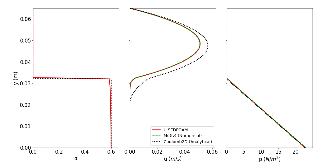
python plot_tuto1DBedLoadCLB.py
and you should see the following figures:
Extension to the Mu(Iv) rheology
The same configuration can be run using the rheology by modifying the endTime from 350 to 450 in system/controlDict file:
endTime 450;
and the constant/granularRheologyProperties file in the following way:
//FrictionModel  Coulomb;
FrictionModel  MuIv;
And run the code again using the command:
sedFoam_rbgh > log2&
At the end of the run, the results can be post-processed using the python script:
python plot_tuto1DBedLoadMUI.py
that lead to the following figures:
1DAvalancheMuI: Dry granular avalanche
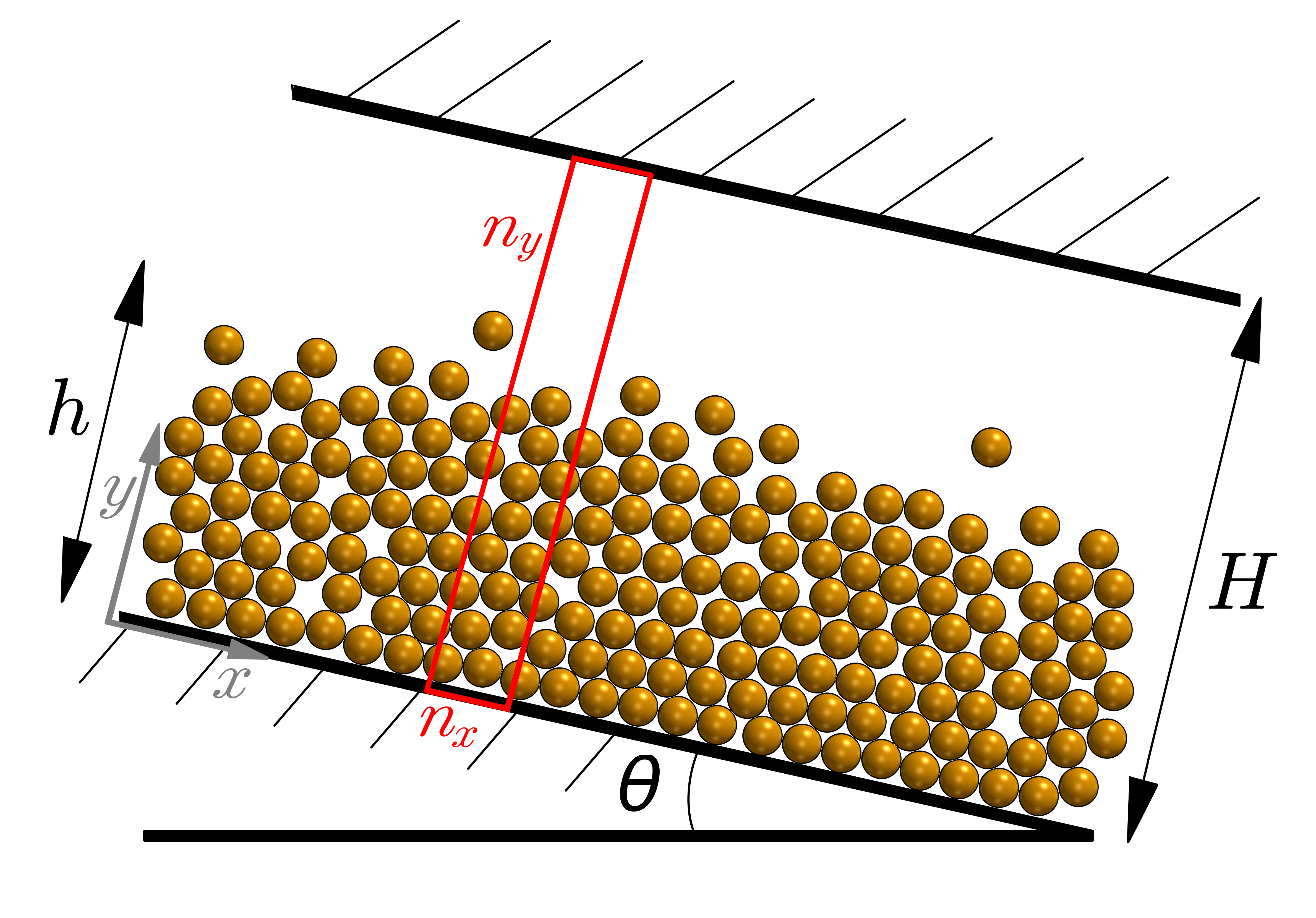
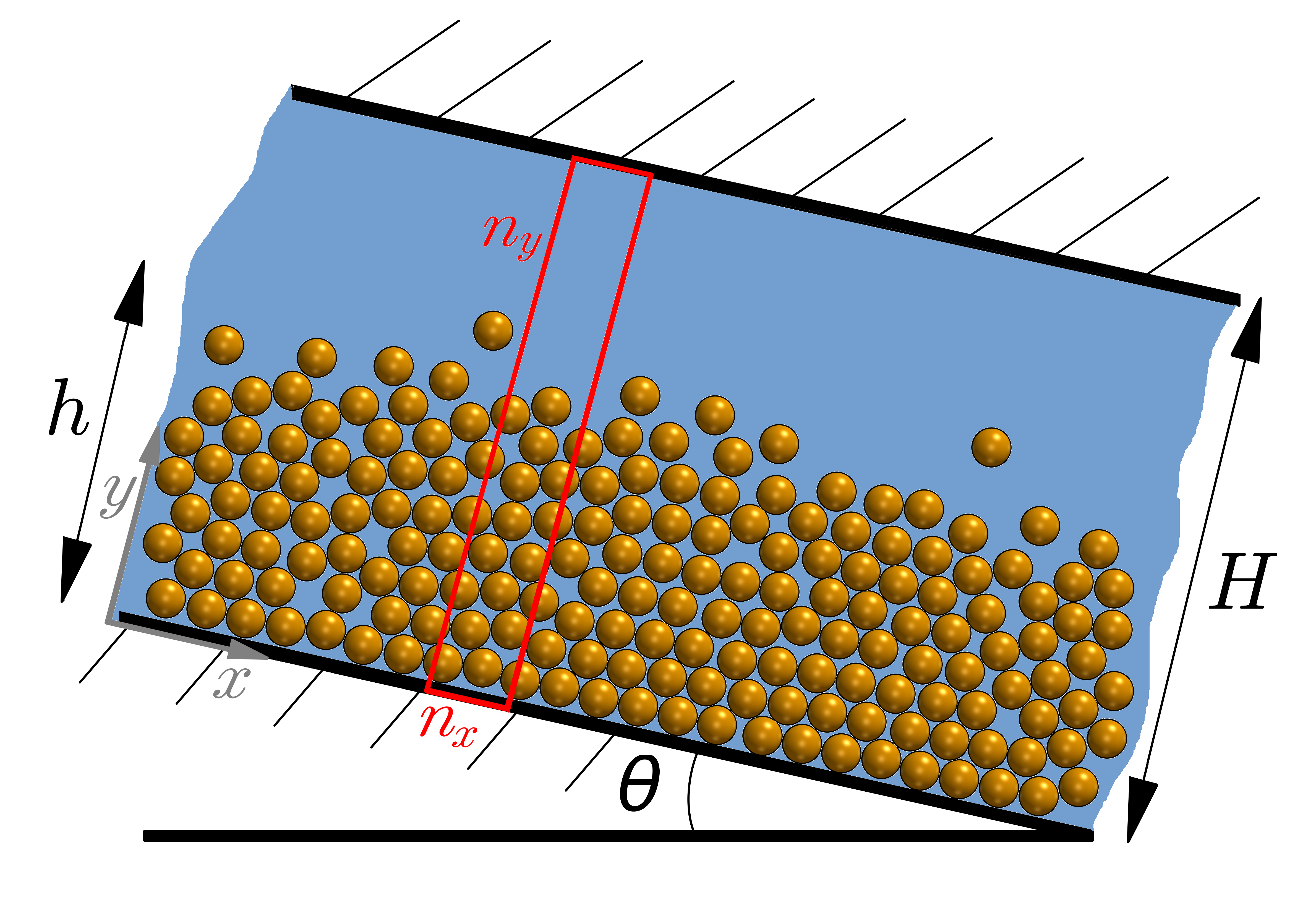
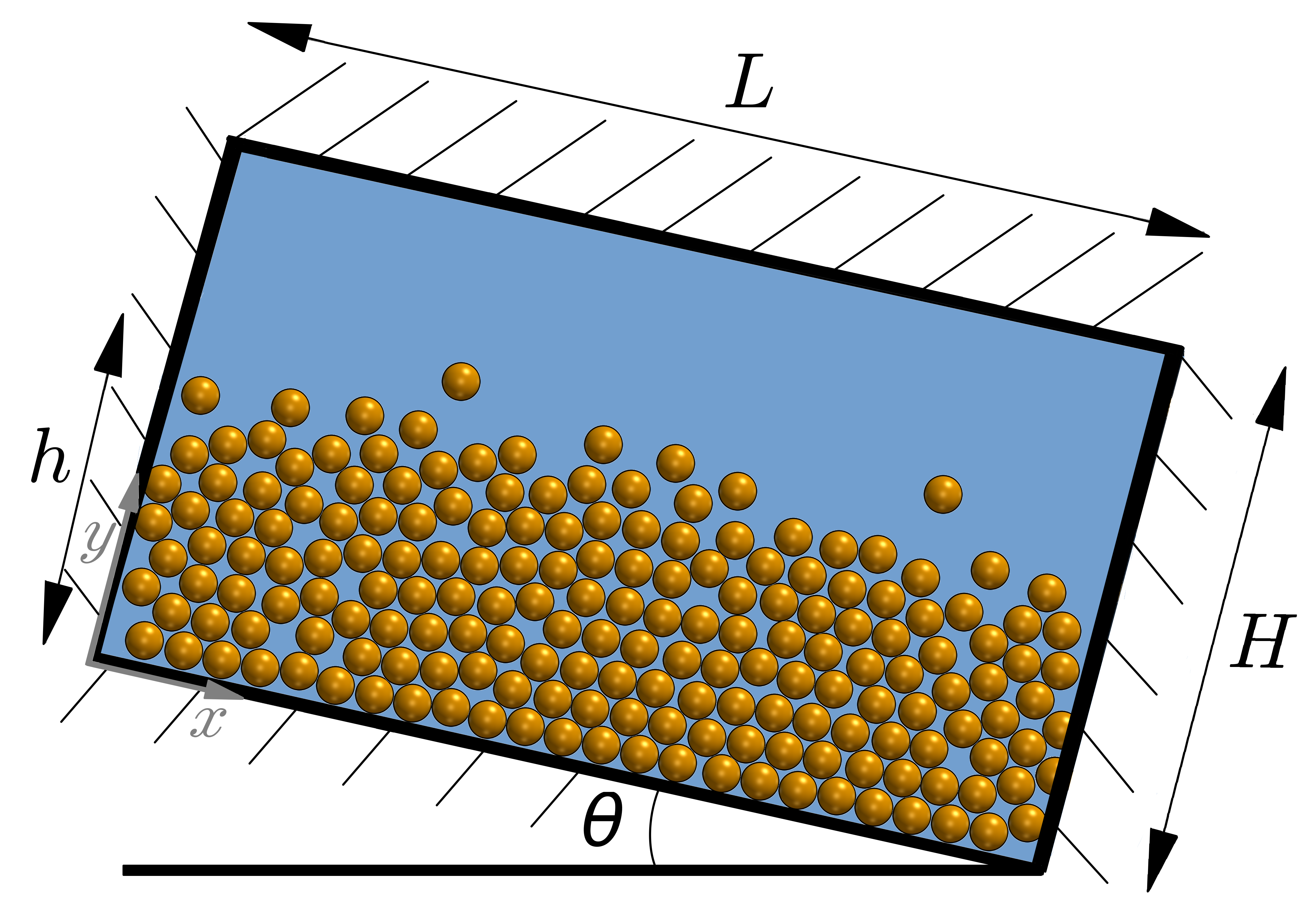
We consider a fluid-solid mixture avalanche flowing under a steady-state moving down a planar slope as illustrated in figure 7. In this example, dense granular flow is reproduced by means of the dense granular flow rheology . Numerical results are contrasted with the analytical solution (Bagnold's solution).
Pre-processing
This tutorial is distributed with sedFoam under the folder sedFoamDirectory/tutorials/laminar/1DAvalancheMuI.
Mesh generation
Because the avalanche is assumed to be in a stationary state, the simulation can be easily reduced to a one-dimensional problem. The numerical domain consists of a rectangle of side length L = 0.01 made dimensionless by the domain size in the x-y plane and of height h=1 in the vertical direction z.
A uniform mesh of 1 by 1 by 100 cells will be used (see =1 and =100 in figure 7). The block structure is the same as for the Sedimentation test case shown in figure 1.
The mesh is generated by running blockMesh within the case directory:
blockMesh
Boundary and initial conditions
The case is set up to start at time t = 0 s, again the initial field data are stored in a 0_org sub-directory of the case directory. The 0_org sub-directory contains several files: alpha.a, U.a, U.b, p_rbgh, muI, pa, Theta, one for each of the solid phase volume fraction (alpha.a), velocities of solid and fluid phases (U.a and U.b), the reduced pressure (p_rbgh) fields whose initial values and boundary conditions must be set. No-slip boundary conditions are imposed for both phases at the top and bottom boundaries (zero velocity at the solid boundaries). Additionally, cyclic boundaries are considered in the inlet and outlet (upstream and downstream boundaries in figure 7.). Cyclic boundaries are imposed to connect two equal meshes. The frontAndBack patch represents the front and back planes of the 2D case and therefore must be set as empty.
Physical properties
The following variables are considered:
| Properties | Value |
|---|---|
| Solid density | |
| Fluid density | |
| Fluid viscosity | |
| Mean particle diameter | |
| Slope inclined at the angle | |
| Solid phase thickness | |
| Initial solid volume fraction |
The transportProperties file for the 1DAvalancheMuI case is shown below:
phasea
{
    rho             rho [ 1 -3 0 0 0 ] 1;
    nu              nu [ 0 2 -1 0 0 ] 1e-6;
    d               d [ 0 1 0 0 0 0 0 ] 0.02;
}

phaseb
{
    rho             rho [ 1 -3 0 0 0 ] 1e-3;
    nu              nu [ 0 2 -1 0 0 ] 1e-1;
    d               d [ 0 1 0 0 0 0 0 ] 1;
}
//*********************************************************************** //
transportModel  Newtonian;

nu              nu [ 0 2 -1 0 0 0 0 ] 1e-1;

// Diffusivity for mass conservation resolution (avoid num instab around shocks)
alphaDiffusion  alphaDiffusion [0 2 -1 0 0 0 0] 0e0;

nuMax           nuMax [0 2 -1 0 0 0 0] 1e2;      // viscosity limiter for the Frictional model (required for stability)

alphaSmall      alphaSmall [ 0 0 0 0 0 0 0 ] 1e-6;  // minimum volume fraction (phase a) for division by alpha
Dense granular flow rheology is used as shown in granularRheologyProperties:
granularRheology   on;

granularDilatancy  off;

granularCohesion off;

alphaMaxG       alphaMaxG [ 0 0 0 0 0 0 0 ] 0.6;

mus             mus  [ 0 0 0 0 0 0 0 ] 0.38;

mu2             mu2  [ 0 0 0 0 0 0 0 ] 0.64;

I0              I0  [ 0 0 0 0 0 0 0 ] 0.3;

Bphi            Bphi [ 0 0 0 0 0 0 0 ] 0.31;

n               n [ 0 0 0 0 0 0 0 ] 2.5;

BulkFactor      BulkFactor [ 0 0 0 0 0 0 0 ] 0e0;

PaMin           PaMin [ 0 0 0 0 0 0 0 ] 1e-6;

relaxPa         relaxPa [ 0 0 0 0 0 0 0 ] 1;

tau_inv_min     tau_inv_min [ 0 0 -1 0 0 0 0 ] 1e-3;

FrictionModel   MuI;

PPressureModel  MuI;

FluidViscosityModel  none;
Additionally, FluidViscosityModel model is set to none. Even though no FluidViscosityModel is specified, the shear induced contribution associated to the fluid phase is still present. However, it has insignificant influence on the results due to the low fluid viscosity. On the contrary, the analytical solution assumes that the shear induced contribution to the fluid phase is null.
Finally, the file constant/g is modified to take into account the and -axis component of gravity with magnitude . In this work the plane is inclined to , however, other angles may be considered.
dimensions      [0 1 -2 0 0 0 0];

// tilt angle = 26 deg
value           (0.43837 -0.89879 0);
Post-processing using python
The analytical and SedFoam results are obtained running the python script plot_tuto1DAvalancheMuI.py located in the folder tutorials/Py:
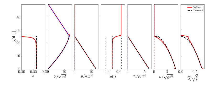
python plot_tuto1DAvalancheMuI.py
and you should see the following figure:
1DWetAvalancheMuIv: Immersed granular avalanche
We consider a fluid-solid mixture avalanche flowing under a steady-state moving down a planar slope as illustrated in figure 9. In contrast to previous tutorial, the granular material is immersed in a viscous fluid. Therefore, dense granular flow rheology is used instead. Additionally, dilatancy effects are included in this example. Iverson et al.(2000) showed the initial dynamics of underwater avalanches strongly depend on the initial volume fraction: initially loose granular beds are instantaneously mobilized after tilting the plane whereas in initially dense granular beds, the motion of the avalanche is delayed. This mechanism is accompanied by an expansion (initially dense) or contraction (initially loose) of the granular medium that modifies the pore space. Consequently, negative (dense packings) or positive (loose packings) excess pore pressures develop within the mixture. In this example, we reproduce a dense granular avalanche in 1D. In order to reach an initial equilibrium state, 200 seconds are required to let the granular layer deposit by gravity.
Pre-processing
This tutorial is distributed with SedFoam under the folder sedFoamDirectory/tutorials/laminar/1DWetAvalanche.
Physical properties
The following variables are considered to reproduce the experimental results of Pailha et al. (2008):
| Properties | Value |
|---|---|
| Solid density | |
| Fluid density | |
| Fluid viscosity | |
| Mean particle diameter | |
| Slope inclined at the angle | |
| Solid phase thickness | |
| Initial solid volume fraction |
The transportProperties file for the 1DWetAvalancheMuIv case is shown below:
phasea
{
    rho             rho [ 1 -3 0 0 0 ] 2500;
    nu              nu [ 0 2 -1 0 0 ] 1e-6;
    d               d [ 0 1 0 0 0 0 0 ] 160.e-6;
}

phaseb
{
    rho             rho [ 1 -3 0 0 0 ] 1041.;
    nu              nu [ 0 2 -1 0 0 ] 9.221902017291067e-05;
    d               d [ 0 1 0 0 0 0 0 ] 2.e-3;
}
//*********************************************************************** //
transportModel  Newtonian;

nu              nu [ 0 2 -1 0 0 0 0 ] 9.221902017291067e-05;

// Diffusivity for mass conservation resolution (avoid num instab around shocks)
alphaDiffusion  alphaDiffusion [0 2 -1 0 0 0 0] 0e-8;

nuMax           nuMax [0 2 -1 0 0 0 0] 1e0;      // viscosity limiter for the Frictional model (required for stability)

alphaSmall      alphaSmall [ 0 0 0 0 0 0 0 ] 1e-6;  // minimum volume fraction (phase a) for division by alpha
Sedimentation process
Dense granular flow rheology is used as shown in granularRheologyProperties. The dilatancy model is switched off during the sedimentation process:
granularRheology   on;

granularDilatancy  on;

granularCohesion off;

alphaMaxG       alphaMaxG [ 0 0 0 0 0 0 0 ] 0.62;

mus             mus  [ 0 0 0 0 0 0 0 ] 0.425;

mu2             mu2  [ 0 0 0 0 0 0 0 ] 0.765;

I0              I0  [ 0 0 0 0 0 0 0 ] 0.004;

Bphi            Bphi [ 0 0 0 0 0 0 0 ] 1.0;

n               n [ 0 0 0 0 0 0 0 ] 2.5;

Dsmall          Dsmall [ 0 0 -1 0 0 0 0 ] 1e-6;

BulkFactor      BulkFactor [ 0 0 0 0 0 0 0 ] 0e0;

relaxPa         relaxPa [ 0 0 0 0 0 0 0 ] 1.0;

K_dila          K_dila [ 0 0 0 0 0 0 0 ] 0.0;

alpha_c         alpha_c [ 0 0 0 0 0 0 0 ] 0.585;

FrictionModel   MuIv;

PPressureModel  MuIv;

FluidViscosityModel  BoyerEtAl;
If you wish a different initial volume fraction you need to adjust the 0_org/alphaPlastic file accordingly. Reference values: alphaPlastic=0.575 leads to , alphaPlastic=0.545 leads to and alphaPlastic=0.520 leads to .
Launching the 1D immersed avalanche
After 200 seconds of sedimentation, the file constant/g should be adjusted to reproduce the inclined plane (25 degrees slope):
dimensions      [0 1 -2 0 0 0 0];
// tiltangle = 25°
value           ( 4.14588187090559 -8.8908809188120586 0 );
The dilatancy model is turn on in granularRheologyProperties to reproduce the coupling between the dilatancy and the pore pressure feedback. The dilatancy prefactor in this example is set to :
K_dila K_dila [ 0 0 0 0 0 0 0 ] 4.0;
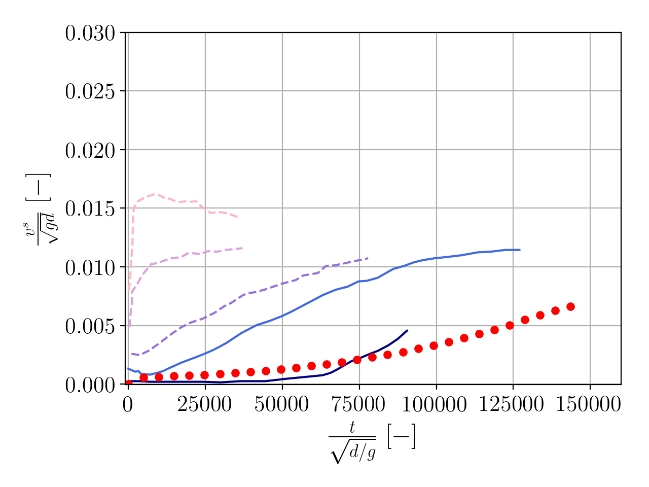
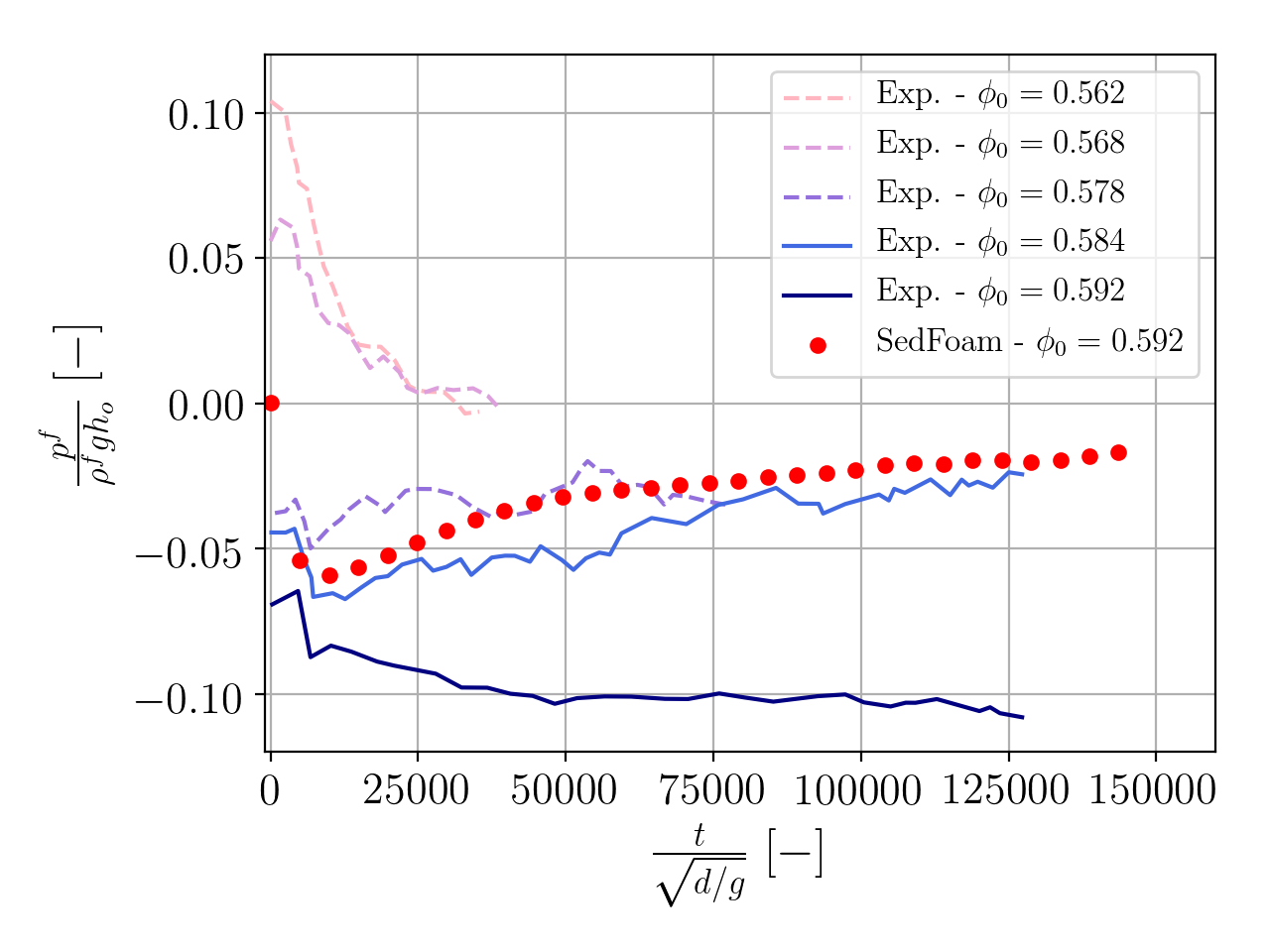
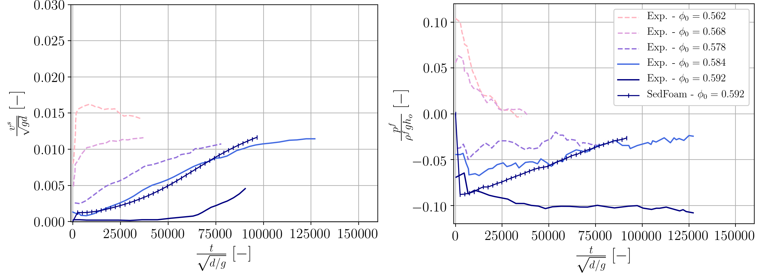
Post-processing using python
The SedFoam and Pailha et al. (2008) experimental results are obtained running the python script plot_tuto1DWetAvalanche.py located in the folder tutorials/Py:
python plot_tuto1DWetAvalanche.py
and you should see the following figure:
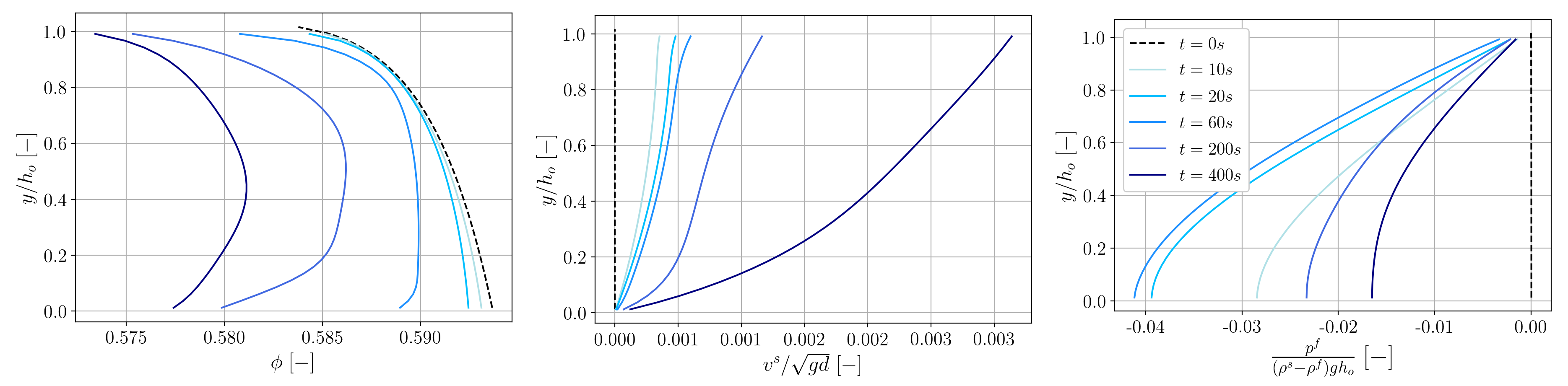
In order to illustrate the dilatant effects and the pore pressure feedback mechanism of the avalanche we run the python script plot_tuto1DWetAvalancheVerticalProfiles.py. The resulting figure is depicted below. We observe the evolution of the volume fraction, particle velocity and excess of pore pressure along the vertical axis.
2DWetAvalancheMuIv: Immersed granular avalanche
We consider a layer of granular material fully immersed in a viscous liquid. The granular layer is inclined so it starts moving down a planar slope as illustrated in figure 13. The geometrical parameters and boundary conditions are set to reproduce precisely the experimental setup of Pailha et al.(2008). In this example, the dense granular flow rheology is considered. Additionally, dilatancy effects are included to better reproduce the initial dynamics of the granular flow. Iverson et al.(2000) showed the initial dynamics of underwater avalanches strongly depend on the initial volume fraction: initially loose granular beds are instantaneously mobilized after tilting the plane whereas in initially dense granular beds, the motion of the avalanche is delayed. This mechanism is accompanied by an expansion (initially dense) or contraction (initially loose) of the granular medium that modifies the pore space. Consequently, negative (dense packings) or positive (loose packings) excess pore pressures develop within the mixture. In this example, we reproduce a dense granular avalanche in 2D. In order to reach an initial equilibrium state, 200 seconds are required to let the granular layer deposit by gravity. In order to save up some computational time, the deposition process is carried out in a 1D simulation in the Reference1D directory.
Pre-processing
This tutorial is distributed with SedFoam under the folder sedFoamDirectory/tutorials/laminar/2DWetAvalanche.
1D Deposition process
The 1D sedimentation test can be launched by executing Allrun in the Reference1D directory.
If you want a different initial volume fraction you need to adjust the 0_org/alphaPlastic file accordingly. Reference values: alphaPlastic=0.575 leads to , alphaPlastic=0.545 leads to and alphaPlastic=0.520 leads to .
Mesh generation
The numerical domain consists of a rectangle of side length in the x-z plane and height in the vertical direction. The initial bed depth is . The mesh consists of 1000 elements in the horizontal direction and 70 elements in the vertical direction. The meshing utility snappyHexMesh is executed to generate a finer mesh in regions of high concentration.
The meshing and refinement process are generated by running:
blockMesh
snappyHexMesh -overwrite
extrudeMesh
Boundary and initial conditions
Unlike previous tutorials, this case is set up to start at time t = 200s, time enough to reproduce an initially dense granular bed by a 1D deposition test. The initial fields are retrieved from Reference1D directory and transformed to the new 2D geometry by means of the mapFields utility:
# create the initial time folder
cp -r 0_org 200

# Initialize fields
mapFields -sourceTime 200 Reference1D
In order to reproduce the experimental setup of Pailha et al. (2008), all the x-y plane boundaries are set as wall boundaries. The velocities of both phases are set to zero at all boundaries (lateral, top and bottom) while a fixedFluxPressure condition is imposed for the excess pore pressure on all boundaries. An homogeneous Neumann boundary condition (zero gradient) is imposed for all the other quantities.
Physical properties
The following variables are considered to reproduce the experimental results of Pailha et al. (2008):
| Properties | Value |
|---|---|
| Solid density | |
| Fluid density | |
| Fluid viscosity | |
| Mean particle diameter | |
| Slope inclined at the angle | |
| Solid phase thickness | |
| Box length | |
| Box height | |
| Initial solid volume fraction |
Dense granular flow rheology and the dilatancy model is used as shown in granularRheologyProperties:
granularRheology   on;

granularDilatancy  on;

granularCohesion off;

alphaMaxG       alphaMaxG [ 0 0 0 0 0 0 0 ] 0.62;


mus             mus  [ 0 0 0 0 0 0 0 ] 0.425;

mu2             mu2  [ 0 0 0 0 0 0 0 ] 0.765;

I0              I0  [ 0 0 0 0 0 0 0 ] 0.004;

Bphi            Bphi [ 0 0 0 0 0 0 0 ] 1.0;

n               n [ 0 0 0 0 0 0 0 ] 2.5;

Dsmall          Dsmall [ 0 0 -1 0 0 0 0 ] 1e-6;

BulkFactor      BulkFactor [ 0 0 0 0 0 0 0 ] 0e0;

relaxPa         relaxPa [ 0 0 0 0 0 0 0 ] 0.01;

K_dila          K_dila [ 0 0 0 0 0 0 0 ] 4.0;

alpha_c         alpha_c [ 0 0 0 0 0 0 0 ] 0.585;

FrictionModel   MuIv;

PPressureModel  MuIv;

FluidViscosityModel  BoyerEtAl;
Computation launching
Like in previous case, you can launch the computation by executing Allrun. The simulations will run in parallel on 18 cores.
# Decompose the case and run in parallel
decomposePar
mpirun -np 18 sedFoam_rbgh -parallel > log&
Post-processing using python
You just have to run the python script plot_tuto2DWetAvalanche.py located in the folder tutorials/Py:
python plot_tuto2DWetAvalanche.py
and you should see the following figures:
2DCollapse: Granular column collapses
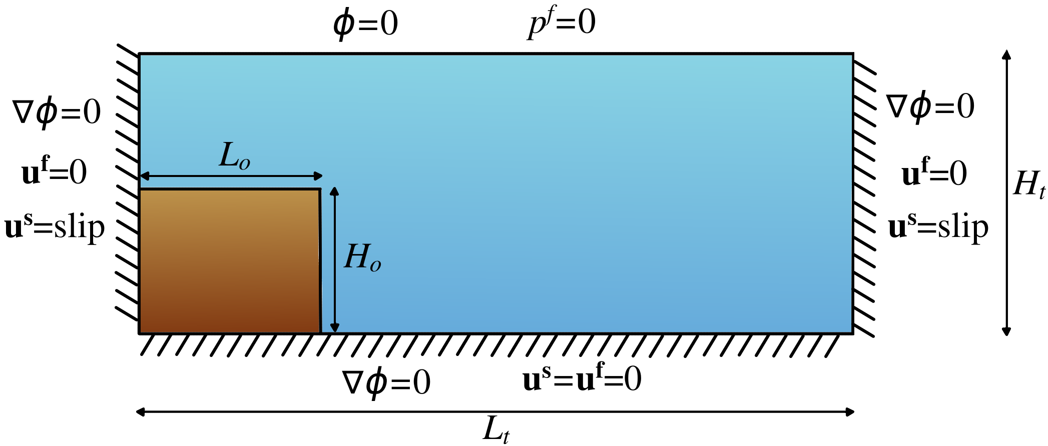
In this section,sedFoam is used to reproduce initially loose and dense granular column collapses. More specifically, this section consists of reproducing the experimental granular collapses of Rondon et al. (2011). The granular column collapse is used to extend the dilatancy model to a more complex and realistic configuration. Numerical results are published in the work of Montellà et al (2023).
The experiments performed by Rondon et al. (2011). investigated the collapse of a granular column in a viscous liquid. Initially dense columns resulted in negative pore pressures that slowed down the collapse, while in loose granular packings, the collapsing process was triggered instantaneously with positive pore pressures that enhanced a rapid flow. Although several volume fractions and aspects ratios were analyzed, only two representative cases (an initially loose column with and an initially dense packing with ) will be considered in this work. The experimental setup consisted of a tank with a length of , and a width and height of . A removable gate was placed vertically and glass beads were poured behind the gate. During the experiments, the excess of pore pressure was measured at the bottom at from the left side of the tank. The numerical setup is presented in the following figure:
Pre-processing
This tutorial is distributed with SedFoam under the folder sedFoamDirectory/tutorials/laminar/2DCollapse/ . Inside that folder you can find two cases, the loose and the dense scenarios.
1D Deposition process
The 1D sedimentation to prepare the loose and dense cases can be launched by executing Allrun in the initial_1D_profile/1DSedim/ directory.
Initial conditions
The initial fields are retrieved from initial_1D_profile/1DSedim/ directory and transformed to the new 2D geometry by means of the mapFields utility:
# create the initial time folder
cp -r 0_org 0
# Initialize fields
mapFields -sourceTime 400 initial_1D_profile/1DSedim/
Physical properties
The following variables are considered to reproduce the experimental results of Rondon et al. (2023):
| Properties | Value |
|---|---|
| Solid density | |
| Fluid density | |
| Fluid viscosity | |
| Mean particle diameter |
Dense granular flow rheology and the dilatancy model is used as shown in granularRheologyProperties:
granularRheology   on;

granularDilatancy on;

granularCohesion  off;

alphaMaxG       alphaMaxG [ 0 0 0 0 0 0 0 ] 0.625;

mus             mus  [ 0 0 0 0 0 0 0 ] 0.425;

mu2             mu2  [ 0 0 0 0 0 0 0 ] 0.765;

I0              I0  [ 0 0 0 0 0 0 0 ] 0.004;

Bphi            Bphi [ 0 0 0 0 0 0 0 ] 1.;

n               n [ 0 0 0 0 0 0 0 ] 2.5;

Dsmall          Dsmall [ 0 0 -1 0 0 0 0 ] 1e-6;

BulkFactor      BulkFactor [ 0 0 0 0 0 0 0 ] 0e0;

K_dila      K_dila [ 0 0 0 0 0 0 0 ] 40;

alpha_c      alpha_c [ 0 0 0 0 0 0 0 ] 0.57;

relaxPa         relaxPa [ 0 0 0 0 0 0 0 ] 1e-0;

FrictionModel   MuIv;

PPressureModel  MuIv;

FluidViscosityModel BoyerEtAl;
Computation launching
You can launch the computation by executing Allrun. The simulations will run in parallel on 4 cores.
# Decompose the case and run in parallel
decomposePar
mpirun -np 4 sedFoam_rbgh -parallel > log&
Post-processing using python
You just have to run the python script plot_tuto2DCollapse.py located in the folder tutorials/Py. You will need to launch both loose and dense cases before running the script.
python plot_tuto2DCollapse.py
and you should see the following figures:
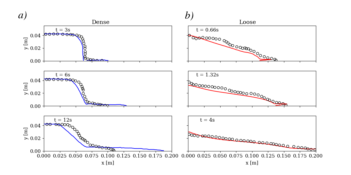
It is worth mentioning that the numerical cases have been significantly coarsened to obtain the results rapidly and illustrate the potential of the dilatancy model. We refer the reader to Montellà et al. (2023) for more detailed data and a thorough analysis.