Reynolds-averaged flow tutorials
In this chapter multi-dimensional test cases are presented to illustrate the full SedFoam capabilities to deal with complex geometries as well as to provide configuration files to allow for the development of new configurations.
1DBoundaryLayer: Single-phase turbulent boundary layer flow
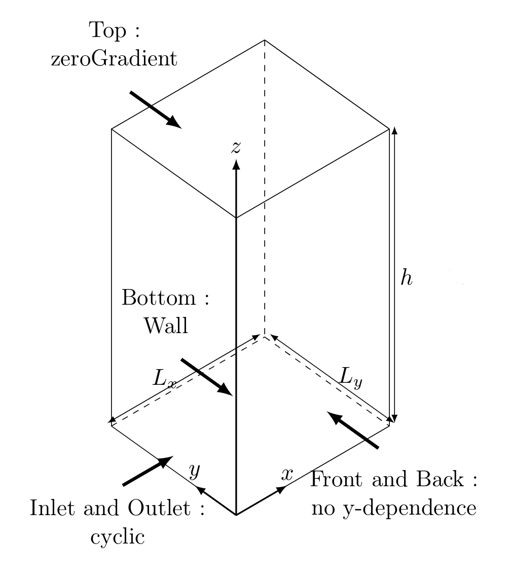
In this test case, tturbulence model k-omega (Wilcox, 1988) is validated for a single-phase boundary layer flow over a smooth surface. The numerical results are compared with the DNS results of Moser et al. (1999). A water column of dimensionless height is moving over a flat plate driven by a pressure gradient imposed along the x-axis. In this configuation, there are no sediments and the volumetric concentration of particles is set to alpha=0. A sketch of the 1D vertical computational domain is presented below:
This tutorial is distributed with sedFoam under the folder sedFoamDirectory/tutorials/RAS/1DBoundaryLayer.
The domain is divided in 64 elements, with a cell expansion ratio of 1.026 along the vertical direction (the ratio between the first cell and the last cell is equal to 10). For such mesh the normalized distance to the wall from the first cell is with the bottom friction velocity and the fluid viscosity.
The physical properties are chosen to obtain a dimensionless solution with , . The parameters are set in the file constant/transportProperties and ar given as follows:
// * * * * * * * * * * * * sediment properties * * * * * * * * * * * * //
phasea
{
    rho             rho [ 1 -3 0 0 0 ] 1;
    nu              nu [ 0 2 -1 0 0 ] 0e0;
    d               d [ 0 1 0 0 0 0 0 ] 1.e-7;
    sF              sF   [ 0 0  0 0 0 0 0 ] 1;
    hExp            hExp [ 0 0  0 0 0 0 0 ] 2.65;
}

phaseb
{
    rho             rho [ 1 -3 0 0 0 ] 1;
    nu              nu [ 0 2 -1 0 0 ] 7.2727e-5;
    d               d [ 0 1 0 0 0 0 0 ] 3.e-3;
    sF              sF   [ 0 0  0 0 0 0 0 ] 0.5;
    hExp            hExp [ 0 0  0 0 0 0 0 ] 2.65;
}
    d [ 0 1 0 0 0 0 0 ] 1;
}
//*********************************************************************** //
The boundary Reynolds number based on the friction velocity in Moser et al. (1999) is, . In sedFoam the flow is driven by a pressure gradient acting as a source term in the momentum equations. The pressure gradient is calculated by integrating the fluid momentum equation along th wall-normal direction sas follows:
and written in the file constant/forceProperties using the keyword gradPMEAN.
Boundary conditions
The inlet and outlet boundaries are set to cyclic while the front and back boundaries are set to empty. The latter boundary condition means that the y-components are not considered by the solver (i.e. 2 velocity components only). At the top boundary, the pressure is fixed to zero and a zero gradient (*i.e* Neumann boundary condition) is imposed on all the other quantities. At the wall, the velocity is set to zero, a zeroGradient condition is imposed for the pressure and a wall function is imposed for the TKE dissipation.
The wall function is prescribing the value of TKE dissipation at the wall to follow the analytical solution from Wilcox (1988). In this tutorial, a rough wall function is used prescribing the value of at the wall following:
with a tuning parameter taking into account bed roughness as follows:
Post-processing using python
The SedFoam results are plotted using the python script plot_tuto1DBoundayLayer.py located in the folder tutorials/Py:
python plot_tuto1DBoundaryLayer.py
and you should see the following figure:
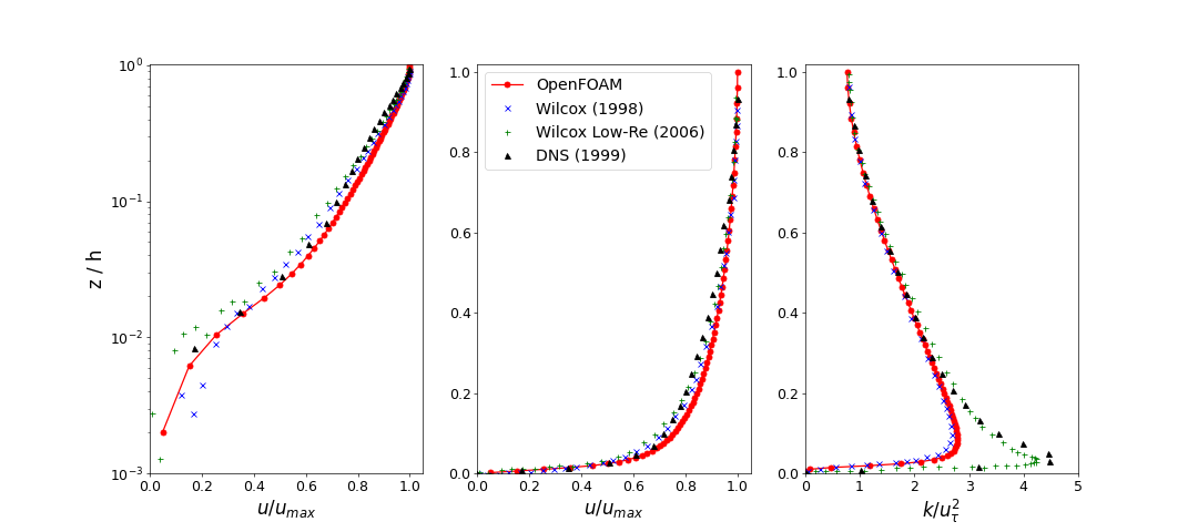
Moser, R. D., Kim, J., and Mansour, N. N. (1999). Direct numerical simulation of turbulent channel flow up to retau=590. Physics of Fluids, 11(4):943-945. Wilcox, D. C. (2008). Formulation of the k-w turbulence model revisited. AIAA Journal, 46(11):2823–2838.
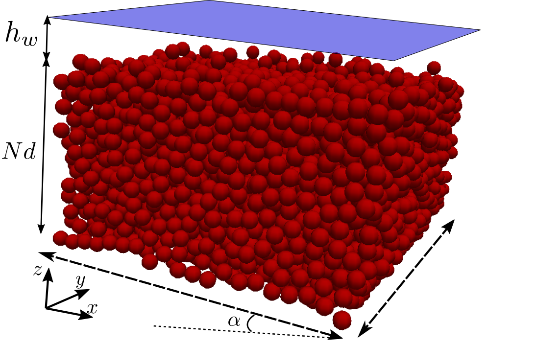
1DBedloadTurb: Turbulent bedload transport
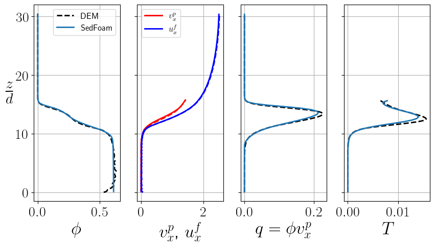
The aim of this tutorial is to explain how to use the kinetic theory to model the sediment phase in turbulent bedload transport. It is based on a comparison coupled fluid-DEM (discrete element method) simulations. In DEM simulations, the motion of each particles is solved individually. The source code is YADE (Smilauer et al. 2015) and the coupling with the fluid phase presented in Maurin et al. (2015). The exact same fluid model is considered in both the fluid-DEM simulations and in the sedfoam simulation (mixing length) in order to focus on the granular flow modelling. Averaged quantities are computed in the DEM (volume fraction, particle velocity, granular temperature, etc.) which will be considered as a basis to compare with the sedFoam simulation. A complete description and analyses of the granular flow modeling with the kinetic theory can be found Chassagne et al. (2023).
Pre-processing
This tutorial is distributed with SedFoam under the folder sedFoamDirectory/tutorials/RAS/1DBedLoadTurb.
Mesh generation
The numerical domain consists of a square of side length L = 0.00147 m in the x-y plane and of height h=0.147 m in the vertical direction z. The side length is chosen to ensure a unity cell aspect ratio. A uniform mesh of 1 by 1 by 120 cells will be used. The block structure is the same as for the Sedimentation test case.
The mesh is generated by running blockMesh from within the case directory:
blockMesh
Boundary and initial conditions
The case is set up to start at time s, again the initial field data are stored in a 0_org sub-directory of the case directory. The 0_org sub-directory contains several files: alpha.a, alphaMinFriction, alphaPlastic, U.a, U.b, p_rbgh, pa, Theta, one for each of the solid phase volume fraction (alpha.a), velocities of solid and fluid phases (U.a and U.b), the reduced pressure (p_rbgh) fields whose initial values and boundary conditions must be set. The initial profile of concentration (in alpha.a) is a hyperbolic tangent whose parameters have been compute so that the exact same amount of granular mass as in the DEM simulation is set in the sedFoam simulation. Compared with the sedimentation test case, no-slip boundary conditions are imposed for both phase velocity at the top and bottom boundaries.
forAll(mesh.C(), i)
{
 scalar y = mesh.C()[i].y();
        alpha_a[i] = 0.305*(1.0+tanh((12.5*0.006-y)/0.005));
}
Physical properties
The transportProperties file for the 1DBedloadTurb case is shown below. The same particle properties as in the DEM are.
// * * * * * * * * * * * * sediment properties * * * * * * * * * * * * //
phasea
{
    rho             rho [ 1 -3 0 0 0 ] 2500;
    nu              nu [ 0 2 -1 0 0 ] 1e-6;
    d               d [ 0 1 0 0 0 0 0 ] 6.e-3;
    sF              sF   [ 0 0  0 0 0 0 0 ] 1;    // shape Factor to adjust settling velocity for non-spherical particles
    hExp            hExp [ 0 0  0 0 0 0 0 ] 3.1;  // hindrance exponent for drag: beta^(-hExp) (2.65 by default)
}
// * * * * * * * * * * * * fluid properties * * * * * * * * * * * * //
phaseb
{
    rho             rho [ 1 -3 0 0 0 ] 1000;
    nu              nu [ 0 2 -1 0 0 ] 1.e-6;
    d               d [ 0 1 0 0 0 0 0 ] 3.e-3;
    sF              sF   [ 0 0  0 0 0 0 0 ] 0.5;
    hExp            hExp [ 0 0  0 0 0 0 0 ] 3.1;
}
//*********************************************************************** //
transportModel  Newtonian;

nu              nu [ 0 2 -1 0 0 0 0 ] 1.e-6;

nuMax           nuMax [0 2 -1 0 0 0 0] 1e2;      // viscosity limiter for the Frictional model (required for stability)

alphaSmall      alphaSmall [ 0 0 0 0 0 0 0 ] 1e-5;  // minimum volume fraction (phase a) for division by alpha

// ************************************************************************* //
The fluid and particles are submitted to gravity. This is accounted for as a pressure gradient source term in the momentum conservation equations. It corresponds to gradPMEAN in file forceProperties with , with (kg/s), (m/s^2) and . The tilt parameter is set to 1, so that the source term in the granular momentum equation is automatically set to .
// * * * * * * * * * * * * * following are for presure * * * * * * * * * * * * * * * //
gradPMEAN        gradPMEAN        [ 1 -2 -2 0 0 0 0 ] (490.5 0 0 ); // mean pressure

tilt             tilt             [ 0  0  0 0 0 0 0 ] 1; // To impose same gravity term to both phases

Cvm             Cvm [ 0 0 0 0 0 ] 0;                // Virtual/Added Mass coefficient

Cl              Cl [ 0 0 0 0 0 ] 0;                 // Lift force coefficient

Ct              Ct [ 0 0 0 0 0 ] 0;                 // Eddy diffusivity coefficient for phase a

debugInfo       true;

writeTau        true;

// * * * * * * * * * * * * end of definition of pressure * * * * * * * * * * * * * //
The fluid turbulence is modelled with a mixing length approach with the same parameters as in the DEM fluid model (expoLM=1, kappaLM=0.41, alphaMaxLM=0.61) :
// * * * * * * * * * * * * * * * * * * * * * * * * * * * * * * * * * * * * * //
simulationType  RAS;

RAS{
RASModel        twophaseMixingLength;
//RASModel        twophasekEpsilon;
//RASModel        twophasekOmega;

turbulence      on;
printCoeffs     on;

twophaseMixingLengthCoeffs
{
expoLM 1.0;
alphaMaxLM 0.61;
kappaLM 0.41;
}
}
// ************************************************************************* //
In the dictionary interfacialProperties file the drag model from DallaValle is used (as in the DEM).
Kinetic theory will be used to compute the kinetic contributions of granular stresses. Be sure to set granularRheology to off in granularRheologyProperties. The kineticTheoryProperties file contains all information to set up thze kinetic theory model. First, particle properties have to be given, restitution coefficient and interparticle friction . alphaMax is the maximum packing fraction and phi is the angle of repose, below which the granular flow stops moving. This angle depends on the interparticle friction and an empirical formula to compute phi is given in Chassagne et al. (2023) (Appendix). killJ2_, allows to account for (0) or neglect (1) any transfer of fluctuating energy from the fluid to the particles. quadraticCorrectionJ1_ allows you to account for (1) or neglect (0) additional dissipation of granular temperature by the drag force, due to the quadratic nature of drag force in turbulent flows. Then you have to choose which model to use for each of the coefficient of the kinetic theory. The models used in this tutorial correspond to the model developed in Chassagne et al. (2023). The Garzo and Dufty (1999) coefficients are used for the viscosity, conductivity and pressure coefficient. The pressure coefficient of Lun et al. (1984) is the same as the one of Garzo and Dufty (1999). A saltation model can be specified (none by default). This modifies the viscosity and conductivity coefficients in the dilute part of the granular flow to account for saltation motions. In the current version of the code, only the GarzoDufty models can be coupled with a saltation model. The Chialvo & Sundaresan (2013) radial distribution function is used, and it is the only one that accounts for the effect of the interparticle friction coefficient (Chassagne et al. (2013)).
// * * * * * * * * * * * * * * * * * * * * * * * * * * * * * * * * * * * * * //

kineticTheory   on;

limitProduction off;

extended        off;

e               e [ 0 0 0 0 0 0 0 ] 0.7;

muPart          muPart [ 0 0 0 0 0 0 0 ] 0.4;

alphaMax        alphaMax [ 0 0 0 0 0 0 0 ] 0.635;

MaxTheta       MaxTheta [ 0 2 -2 0 0 0 0 ] 0.5;

phi             phi [ 0 0 0 0 0 0 0 ] 20.487; //mus = 0.35 = sin(phi*pi/180)

psi             psi [ 0 0 0 0 0 0 0 ] 0.0;

killJ2_       killJ2_ [ 0 0 0 0 0 0 0] 1;

quadraticCorrectionJ1_ quadraticCorrectionJ1_ [ 0 0 0 0 0 0 0 ] 1;

viscosityModel  GarzoDufty;

conductivityModel GarzoDufty;

granularPressureModel Lun;

saltationModel  Jenkins;

radialModel     ChialvoSundaresan;

// ************************************************************************* //
Discretisation and linear-solver settings
The numerical schemes and the solvers are the same as in the 1DSedim case.
Control
The system/controlDict file is shown thereafter. The endTime is fixed to 30 s with an output every 5s with an adjustable time step limited to 5e-3 s. The simulation should last around 20 minutes.
application     sedFoam;

startFrom       latestTime;

startTime       0;

stopAt          endTime;

endTime         30;

deltaT          1e-5;

writeControl    adjustableRunTime;

writeInterval   1;

purgeWrite      0;

writeFormat     ascii;

writePrecision  6;

timeFormat      general;

timePrecision   6;

runTimeModifiable on;

adjustTimeStep  on;

maxCo           0.1;

maxAlphaCo      0.1;

maxDeltaT       1e-3;
Post-processing using python
You just have to run the python script plot_tuto1DBedLoadTurb.py located in the folder tutorials/Py:
python plot_tuto1DBedLoadTurb.py
and you should see the following figures:
1DSheetFlow: Turbulent sheet-flows
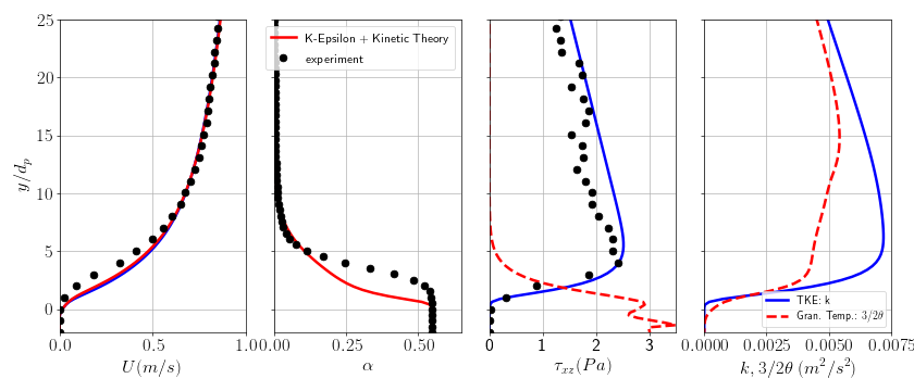
In this tutorial, the turbulent flow over a flat erodible bed drives sediment transport in the intense turbulent bedload tranpsort regime usually referred to as sheet-flow. The results are compared with experimental data from Revil-Baudard et al. (2015). Light-weight non-spherical PMMA particles of median diameter d=3 mm are used having a settling velocity in quiescent water of about m/s. The averaged flow velocity is about U=0.52 m/s corresponding to a bed friction velocity of m/s and a dimensionless bed shear stress, the so-called Shields number , equal to 0.44.
Pre-processing
This tutorial is distributed with sedFoam under the folder sedFoamDirectory/tutorials/RAS/1DSheetFlow.
Mesh generation
The numerical domain consists of a square of side length L = 0.00085 m in the x-y plane and of height h=0.17 m in the vertical direction z. The side length is chosen to ensure a unity cell aspect ratio. A uniform mesh of 1 by 1 by 400 cells will be used. The block structure is the same as for the Sedimentation test case.
The mesh is generated by running blockMesh from within the case directory:
blockMesh
Boundary and initial conditions
The case is set up to start at time t = 0 s, again the initial field data are stored in a 0_org sub-directory of the case directory. The 0_org sub-directory contains several files: alpha.a, alphaMinFriction, alphaPlastic, U.a, U.b, p_rbgh, muI, pa, pa_new, Theta, k.b, epsilon.b, omega.b and nut one for each of the solid phase volume fraction (alpha.a), velocities of solid and fluid phases (U.a and U.b), the reduced pressure (p_rbgh) fields whose initial values and boundary conditions must be set. No-slip boundary conditions are imposed at the bottom and zero gradient at the top for both phase velocities.
Physical properties
The transportProperties file for the 1DSheetFlow case is shown below:
phasea
{
    rho             rho [ 1 -3 0 0 0 ] 1190;
    nu              nu [ 0 2 -1 0 0 ] 0e0;
    d               d [ 0 1 0 0 0 0 0 ] 3.e-3;
    sF              sF   [ 0 0  0 0 0 0 0 ] 0.5;    // shape Factor to adjust settling velocity for non-spherical particles
    hExp            hExp [ 0 0  0 0 0 0 0 ] 2.65;  // hindrance exponent for drag: beta^(-hExp) (2.65 by default)
}

phaseb
{
    rho             rho [ 1 -3 0 0 0 ] 1000;
    nu              nu [ 0 2 -1 0 0 ] 1.e-6;
    d               d [ 0 1 0 0 0 0 0 ] 3.e-3;
    sF              sF   [ 0 0  0 0 0 0 0 ] 0.5;
    hExp            hExp [ 0 0  0 0 0 0 0 ] 2.65;
}
//*********************************************************************** //

transportModel  Newtonian;

nu              nu [ 0 2 -1 0 0 0 0 ] 1.e-6;

nuMax           nuMax [0 2 -1 0 0 0 0] 1e-1;      // viscosity limiter for the Frictional model (required for stability)

alphaSmall      alphaSmall [ 0 0 0 0 0 0 0 ] 1e-6;  // minimum volume fraction (phase a) for division by alpha

alphaAlpha      alphaAlpha [ 0 0 0 0 0 ] 0;         // surface tension
The physical property of the particles (diameter and density) and of the fluid (density and kinematic viscosity) have been set to the experimental values from Revil-Baudard et al. (2015).
Revil-Baudard, T., Chauchat, J., Hurther, D., and Barraud, P.-A. (2015). In- vestigation of sheet-flow processes based on novel acoustic high-resolution velocity and concentration measurements. Journal of Fluid Mechanics, 767:1–30.
In the dictionary interfacialProperties file the drag model from GidaspowSchillerNaumann is used and the shape factor sF is taken to 0.5 to match the settling velocity of a single particle with the measured data (w_fall = 0.056 m/s).
In this tutorial, the kinetic theory is used for the granular stress model and the kineticTheoryProperties reads:
kineticTheory   on;

equilibrium     off;

limitProduction off;

e               e [ 0 0 0 0 0 0 0 ] 0.8;

alphaMax        alphaMax [ 0 0 0 0 0 0 0 ] 0.6;

DiluteCut       DiluteCut [ 0 0 0 0 0 0 0 ] 0.00000;

ttzero          ttzero [ 0 0 1 0 0 0 0 ] 0;

ttone          ttone [ 0 0 1 0 0 0 0 ] 0;

MaxTheta       MaxTheta [ 0 2 -2 0 0 0 0 ] 0.5;

phi             phi [ 0 0 0 0 0 0 0 ] 32.0;

psi             psi [ 0 0 0 0 0 0 0 ] 0.0;

KineticJ1      KineticJ1 [ 0 0 0 0 0 0 0 ] 1; //turn off the viscous dissipation

KineticJ2       KineticJ2 [ 0 0 0 0 0 0 0] 0;

KineticJ3       KineticJ3 [ 0 0 0 0 0 0 0] 0;

viscosityModel  Syamlal;

conductivityModel Syamlal;

granularPressureModel Lun;

frictionalStressModel SrivastavaSundaresan;

radialModel     CarnahanStarling;
The turbulence model is set to kEpsilon in turbulenceProperties:
simulationType  RAS;

RAS{
    RASModel        twophasekEpsilon;

turbulence      on;
printCoeffs     on;
}
Discretisation and linear-solver settings
The numerical schemes and the solvers are the same as in the 1DSedim case except that numerical schemes for the turbulent quantities (k, , ) have been added:
ddtSchemes
{
    default         Euler implicit;
}

gradSchemes
{
    default         Gauss linear;
}

divSchemes
{
    default         none;
// alphaEqn
    div(phi,alpha)  Gauss limitedLinear01 1;
    div(phir,alpha) Gauss limitedLinear01 1;
// UEqn
    div(phi.a,U.a)    Gauss limitedLinearV 1;
    div(phi.b,U.b)    Gauss limitedLinearV 1;
    div(phiRa,Ua)   Gauss limitedLinear 1;
    div(phiRb,Ub)   Gauss limitedLinear 1;
// pEqn
    div(alpha,nu)   Gauss linear;
// k and EpsilonEqn
    div(phi.b,k.b)     Gauss limitedLinear 1;
    div(phi.b,epsilon.b) Gauss limitedLinear 1;
    div(phi.b,omega.b) Gauss limitedLinear 1;
// ThetaEqn
    div(phi,Theta)  Gauss limitedLinear 1;
// alphaPlastic
    div(phia,alphaPlastic)  Gauss limitedLinear01 1;
// pa
    div(phia,pa_new_value)  Gauss limitedLinear 1;
}

laplacianSchemes
{
    default         none;
// UEqn
    laplacian(nuEffa,U.a) Gauss linear corrected;
    laplacian(nuEffb,U.b) Gauss linear corrected;
    laplacian(nuFra,U.a)  Gauss linear corrected;
// pEqn
    laplacian((rho*(1|A(U))),p_rbgh) Gauss linear corrected;
// k and EpsilonEqn
    laplacian(DkEff,k.b) Gauss linear corrected;
    laplacian(DkEff,beta) Gauss linear corrected;
    laplacian(DepsilonEff,epsilon.b) Gauss linear corrected;
    laplacian(DepsilonEff,beta) Gauss linear corrected;
    laplacian(DomegaEff,omega.b) Gauss linear corrected;
//ThetaEqn
    laplacian(kappa,Theta) Gauss linear corrected;
    laplacian(kappa2,alpha) Gauss linear corrected;
}

interpolationSchemes
{
    default  linear;
}

snGradSchemes
{
    default         corrected;
}

fluxRequired
{
    default         no;
    p_rbgh               ;
}
Control
The system/controlDict file is modified compared with the laminar bed load test case, the time step is reduced to s and the endTime is reduced to 150 s that is enough for the steady state to be reached.
application     sedFoam;

startFrom      latestTime;

startTime       0;

stopAt          endTime;

endTime         150;

deltaT          2e-4;

writeControl    adjustableRunTime;

writeInterval   10;

purgeWrite      0;

writeFormat     ascii;

writePrecision  6;

writeCompression uncompressed;

timeFormat      general;

timePrecision   6;

runTimeModifiable on;

adjustTimeStep  yes;

maxCo           0.1;

maxAlphaCo      0.1;

maxDeltaT       5e-4;
Post-processing using python
You just have to run the python script plot_tuto1DSheetFlow.py located in the folder tutorials/Py:
python plot_tuto1DSheetFlow.py
and you should see the following figure:
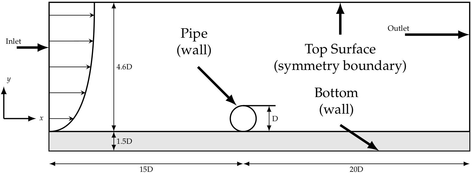
2DPipelineScour: Scour around an horizontal cylinder
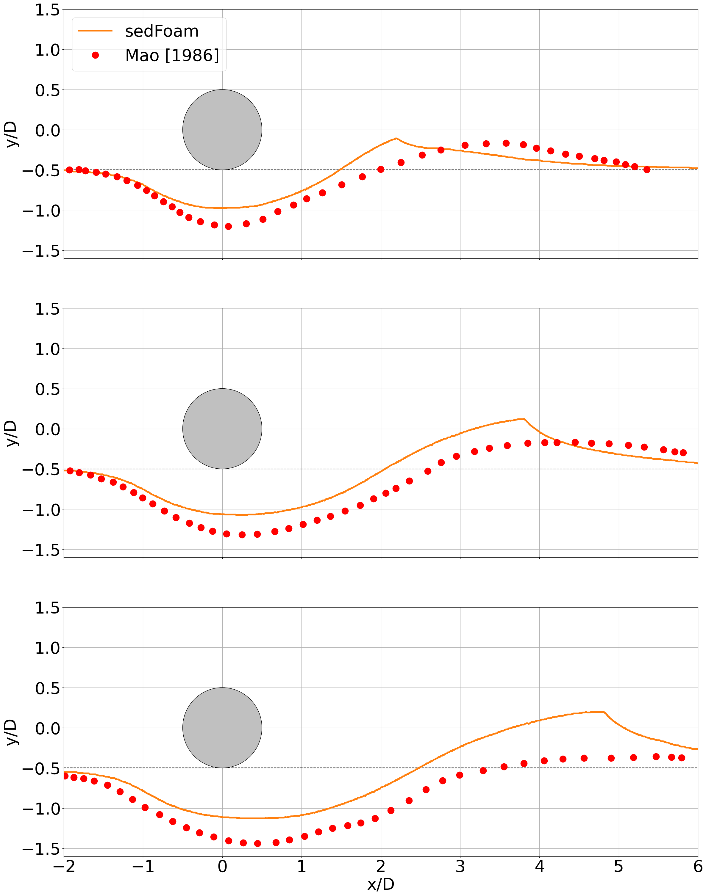
In this tutorial, the experimental configuration investigating scour under a submarine pipeline from Mao (1986) is reproduced numerically.
Pre-processing
This tutorial is distributed with SedFoam under the folder sedFoamDirectory/tutorials/RAS/2DPipelineScour.
Mesh generation
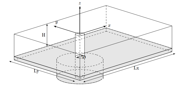
The numerical domain dimensions are presented in figure 7. A cylinder of diameter is placed 15 diameters away from the inlet. The overall domain dimensions were 35 diameters long and 6.1 diameters high. The mesh is generated using the OpenFOAM utilities blockMesh and snappyHexMesh. The mesh generated with blockMesh is a simple rectangle with regular grid spacing excepted in the vertical direction where cells are expanding toward the top boundary. The snappyHexMesh utility uses the file Cyl.stl located in the constant/triSurface directory containing the cylinder geometry to remove mesh cells inside it, add layers of cells around the cylinder and refine cells in regions of high concentration gradient at the bed.
Depending on the turbulence model used, the number of layers should not be the same to accurately predict the boundary layer around the cylinder. The default snappyHexMeshDict in the system directory is written to perform simulations using the turbulence model. For simulations using the model, the user should use/rename the file snappyHexMeshDict_kEpsilon located in the system directory to generate the mesh.
Boundary and initial conditions
The case is set up to start at time t = 0 s, as for the previous tutorials the initial fields data are stored in the 0_org sub-directory of the case directory.
The top boundary condition is a symmetryPlane. The outlet pressure is set to 0. The outlet boundary condition for the velocity is inletOulet corresponding to a homogeneous Neumann boundary condition for outgoing flows and a homogeneous Dirichlet boundary condition for incoming flows. The inlet is decomposed into two parts. From the bottom to , a wall-type boundary condition is applied. From to the top, a rough wall log law velocity profile is used following the expression
with the bottom friction velocity, the von Karman constant and the Nikuradse roughness length. The velocity is increased linearly during the first 4 seconds of the simulation. Inlet values for turbulent quantities were set following , and with the bulk velocity, the distance from the bed to the top boundary and an empirical constant.
The sediment bed is initialised using the expression .
Physical properties
The transportProperties file for the 2DPipelineScour case is shown below:
phasea
{
    rho             rho [ 1 -3 0 0 0 ] 2650;
    nu              nu [ 0 2 -1 0 0 ] 1e-6;
    d               d [ 0 1 0 0 0 0 0 ] 0.36e-3;
    sF              sF   [ 0 0  0 0 0 0 0 ] 1.;    // shape Factor to adjust settling velocity for non-spherical particles
    hExp            hExp [ 0 0  0 0 0 0 0 ] 2.65;  // hindrance exponent for drag: beta^(-hExp) (2.65 by default)
}

phaseb
{
    rho             rho [ 1 -3 0 0 0 ] 1000;
    nu              nu [ 0 2 -1 0 0 ] 1.e-06;
    d               d [ 0 1 0 0 0 0 0 ] 10e-6;
    sF              sF   [ 0 0  0 0 0 0 0 ] 1.;
    hExp            hExp [ 0 0  0 0 0 0 0 ] 2.65;
}
//*********************************************************************** //

alphaSmall      alphaSmall [ 0 0 0 0 0 0 0 ] 1e-4;  // minimum volume fraction (phase a) for division by alpha

alphaAlpha      alphaAlpha [ 0 0 0 0 0 ] 0;         // surface tension

Cvm             Cvm [ 0 0 0 0 0 ] 0;                // Virtual/Added Mass coefficient

Cl              Cl [ 0 0 0 0 0 ] 0;                 // Lift force coefficient


transportModel  Newtonian;

nu              nu [ 0 2 -1 0 0 0 0 ] 1e-06;
nuMax        nuMax [0 2 -1 0 0 0 0] 10;      // viscosity limiter for the Frictional model (required for stability)
The physical property of the particles (diameter and density) and of the fluid (density and kinematic viscosity) have been set to the values given in Mao (1986).
Control
The system/controlDict file indicates that for this case the time step is adaptative to have a maximum Courant number (maxCo) below 0.1 and that the computation ends at 45s of dynamics.
application     sedFoam;

startFrom       latestTime;

startTime       0;

stopAt          endTime;

endTime         45;

deltaT          1.e-4;

writeControl    adjustableRunTime;

writeInterval   0.5;

purgeWrite      0;

writeFormat     binary;

writePrecision  6;

writeCompression false;

timeFormat      general;

timePrecision   6;

runTimeModifiable on;

adjustTimeStep  yes;

maxCo           0.1;

maxAlphaCo      0.3;

maxDeltaT       15.e-5;
Computation launching
As for the previous case, you can launch the computation by executing * Allrun *. The simulations is run in parallel on 16 cores.
Post-processing using python
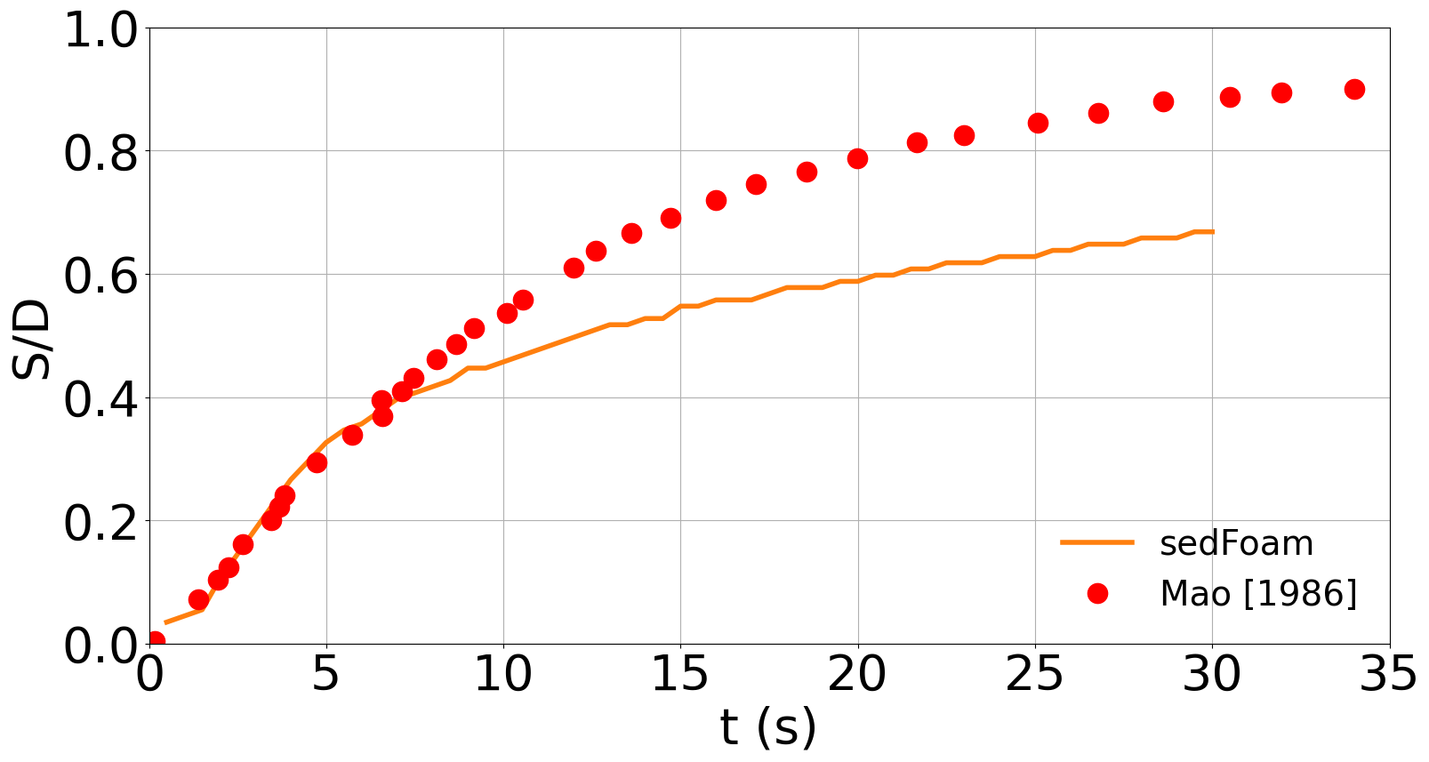
The post-processing python scripts plot_profiles2DPipelineScour.py and plot_depth2DPipelineScour.py are located in the folder tutorials/Py.
The script _profiles2DPipelineScour.py plots bed profiles at 11s, 18s and 25s compared with experimental data like in the following figure:
The script plot_depth2DPipelineScour.py plots the maximum scour depth compared with experimental data like in the following figure:
3DScourCylinder: Scour around a vertical cylinder
In this tutorial, the experimental configuration from Roulund et al (2005) is reproduced numerically.
Pre-processing
This tutorial is distributed with SedFoam under the folder sedFoamDirectory/tutorials/RAS/3DScour.
A 1D boundary layer simulation needs to be run (see folder 1D and Allrun.pre) for fore information. The result of this simulations is then used to intialize the 3D configuation and to impose the inlet boundary condition.
Mesh generation
The numerical domain dimensions are presented in figure 10. A cylinder of diameter is placed 4 diameters away from the inlet. The overall domain dimensions were 13 diameters long, 8 diameters wide and 2 diameters high. The mesh is generated using the OpenFOAM utilities blockMesh and a perl script is used to create the blockMeshDict. A sediment bed layer having a thickness of D/4 is initially set-up except around the cylinder where a scour pit is created with a thickness D and a radius of 2D. The sediments are made of medium sand with median diameter d =0.26 mm and density , the corresponding fall velocity of an individual grain in quiescent water is . The Shields parameter at the inlet and the Reynolds number are the same as is in Roulund et al. (2005), and , respectively. For the sand layer, outside the scour pit, the mesh is composed of 100 vertical levels having a geometric distribution with a common ratio . In the scour pit, an additional 100 grid points are used with a geometric common ratio .
The mesh is generated using the perl script 'generateMeshDict_cyl_3dsedim.pl' using the folowing command:
perl generateMeshDict_cyl_3dsedim.pl 0.4 -0.025 0.0 0.2 -0.1 0.4 1.2 0.8
See the perl script for details about the different parameters.
Boundary and initial conditions
The boundary conditions have to be adapted from the RB case :
(i) At the inlet, vertical profiles obtained from a 1D vertical simulation are imposed for . Zero transverse velocity is prescribed.
(ii) At the outlet, Neumann boundary conditions are specified for all quantities, except for the pressure for which a homogeneous Dirichlet boundary condition is imposed for the reduced pressure. For the velocities, a homogeneous Neumann boundary condition is used when the velocity vector points outside of the domain at the outlet, and a homogeneous Dirichlet boundary condition is used otherwise.
(iii) At the top and side boundaries, the same boundary conditions as in the Rigid-Bed case are used.
(iv) At the walls (including the cylinder), zero velocity (no-slip) is imposed for the three components and a small value is imposed for the turbulent kinetic energy (TKE) k.b. The boundary condition for is specified using the classical wall function from openFOAM at the cylinder and using a constant value is imposed at the bottom.
Physical properties
The following variables are considered to reproduce the experimental results of Pailha et al. (2008):
| Properties | Value |
|---|---|
| Solid density | |
| Fluid density | |
| Fluid viscosity | |
| Mean particle diameter |
The transportProperties file for the 3DScour case is shown below:
phasea
{
    rho             rho [ 1 -3 0 0 0 ] 2650;
    nu              nu [ 0 2 -1 0 0 ] 1e-6;
    d               d [ 0 1 0 0 0 0 0 ] 0.26e-3;
    sF              sF   [ 0 0  0 0 0 0 0 ] 1.;    // shape Factor to adjust settling velocity for non-spherical particles
    hExp            hExp [ 0 0  0 0 0 0 0 ] 2.65;  // hindrance exponent for drag: beta^(-hExp) (2.65 by default)
}

phaseb
{
    rho             rho [ 1 -3 0 0 0 ] 1000;
    nu              nu [ 0 2 -1 0 0 ] 1.e-06;
    d               d [ 0 1 0 0 0 0 0 ] 10e-6;
    sF              sF   [ 0 0  0 0 0 0 0 ] 1.;
    hExp            hExp [ 0 0  0 0 0 0 0 ] 2.65;
}
alphaSmall      alphaSmall [ 0 0 0 0 0 0 0 ] 1e-6;  // minimum volume fraction (phase a) for division by alpha

alphaAlpha      alphaAlpha [ 0 0 0 0 0 ] 0;         // surface tension

Usmall          Usmall [ 0 1 -1 0 0 0 0 ] 1.0e-10;  // minimum friction velocity for local Schmidt calculation

Ufall           Ufall [ 0 1 -1 0 0 0 0 ] 3.44e-2;   //sediment fall velocity


transportModel  Newtonian;

nu              nu [ 0 2 -1 0 0 0 0 ] 1e-06;
nuMax        nuMax [0 2 -1 0 0 0 0] 100;      // viscosity limiter for the Frictional model (required for stability)
The physical property of the particles (diameter and density) and of the fluid (density and kinematic viscosity) have been set to the values given in Roulund et al (2005).
Rheological parameters
The granular stress model is set to granularRheology using the following parameters:
granularRheology   on;

granularDilatancy  off;

granularCohesion off;

alphaMaxG       alphaMaxG [ 0 0 0 0 0 0 0 ] 0.625;

mus             mus  [ 0 0 0 0 0 0 0 ] 0.63;

mu2             mu2  [ 0 0 0 0 0 0 0 ] 1.13;

I0              I0  [ 0 0 0 0 0 0 0 ] 0.6;

Bphi            Bphi [ 0 0 0 0 0 0 0 ] 0.66;

n               n [ 0 0 0 0 0 0 0 ] 2.5;

Dsmall          Dsmall [ 0 0 -1 0 0 0 0 ] 1e-4;

relaxPa         relaxPa [ 0 0 0 0 0 0 0 ] 3e-4;

zbed         zbed [ 0 1 0 0 0 0 0 ] 0.0;

FrictionModel  MuI;

PPressureModel MuI;

FluidViscosityModel  BoyerEtAl;
Control
The system/controlDict file indicates that for this case the time step is adaptative to have a maximum Courant number (maxCo) below 0.5.
Computation launching
As for the previous case, you can launch the computation by executing * Allrun *. The mesh is quite large and at least 100 cores are needed to perform this simulation.
Post-processing using paraview
The post-processing is mostly performed using paraview. No python script is provided withthi configuration at the moment.
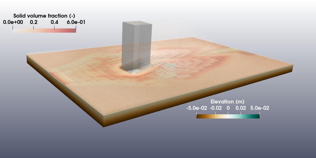
3DScourSqr: Scour around a vertical square cylinder
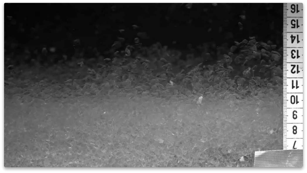
In this tutorial, the hybrid RANS-LES k-omega 2006 SAS is applied to the live-bed configuration of scour around a vertical square cylinder.
Pre-processing
This tutorial is distributed with SedFoam under the folder sedFoamDirectory/tutorials/RAS/3DScourSqr.
Similarly as the 3DScour configuration, a 1D boundary layer simulation needs to be run and then used to intialize the 3D configuation and to impose the inlet boundary condition.
Mesh generation
A square-based cylinder and side is placed 4D away from the inlet. Numerical simulations have been performed with the following computational domain : 12D long, 8D wide and 2,5D high. The mesh is generated using the OpenFOAM utilities blockMesh with Lu, Ld and H the upstream, downstream, width length of the computational domain. A sediment bed layer having a thickness of D/2 is initially set-up. The sediments and hydrodynamics are similar as the 3DScour configuration.
Boundary and initial conditions
The boundary conditions are very close to the 3DScour configuration :
(i) At the inlet, vertical profiles obtained from a 1D vertical simulation are imposed for . Zero transverse velocity is prescribed.
(ii) At the outlet, Neumann boundary conditions are specified for all quantities, except for the pressure for which a homogeneous Dirichlet boundary condition is imposed for the reduced pressure. For the velocities, a homogeneous Neumann boundary condition is used when the velocity vector points outside of the domain at the outlet, and a homogeneous Dirichlet boundary condition is used otherwise.
(iii) At the top and side boundaries, the same boundary conditions as in the 3DScour case are used.
(iv) At the walls (including the cylinder), zero velocity (no-slip) is imposed for the three components and a small value is imposed for the turbulent kinetic energy (TKE) k.b. The boundary condition for is specified using the classical wall function from openFOAM at the cylinder and using a constant value is imposed at the bottom.
Physical properties
The transportProperties file for the 3DScourSqr is identical to the 3DScour configuration.
Kinetic theory
In this tutorial, the kinetic theory is used for the granular stress model and the kineticTheoryProperties reads:
kineticTheory   on;

limitProduction off;

extended        off;

e               e [ 0 0 0 0 0 0 0 ] 0.7;

muPart          muPart [ 0 0 0 0 0 0 0 ] 0.4;

alphaMax        alphaMax [ 0 0 0 0 0 0 0 ] 0.635;

MaxTheta       MaxTheta [ 0 2 -2 0 0 0 0 ] 0.5;

phi             phi [ 0 0 0 0 0 0 0 ] 32;

psi             psi [ 0 0 0 0 0 0 0 ] 0.0;

killJ2_       killJ2_ [ 0 0 0 0 0 0 0] 0;

quadraticCorrectionJ1_ quadraticCorrectionJ1_ [ 0 0 0 0 0 0 0 ] 1;

viscosityModel  GarzoDuftyMod;

conductivityModel GarzoDuftyMod;

granularPressureModel Lun;

saltationModel  none;

radialModel     ChialvoSundaresan;
Turbulence properties
The turbulence model is set to twophasekOmegaSAS in turbulenceProperties.b:
simulationType  RAS;

RAS
{
    RASModel        twophasekOmegaSAS;
    turbulence      on;
    printCoeffs     on;
    twophasekOmegaSASCoeffs
    {
        alphaOmega       0.52;
        betaOmega        0.0708; // original k-omega: 0.072 // k-omega (2006): 0.0708
        C3om             0.35;
        C4om             1.0;
        alphaKomega      0.6; // original k-omega: 0.5 // k-omega (2006): 0.6
        alphaOmegaOmega  0.5;
        Clim             0.875; // original k-omega: 0.0 // k-omega (2006): 0.875
        sigmad           0.125; // original k-omega: 0.0 // k-omega (2006): 0.125
        Cmu              0.09;
        KE2              1.0; //turb modulation
        KE4              1.0; //density stratification g
        nutMax           5e-3;
        popeCorrection   true;

        delta           vanDriest;
        vanDriestCoeffs
        {
            delta           cubeRootVol;
            cubeRootVolCoeffs
            {
                deltaCoeff      1;
            }
            Aplus           26;
            Cdelta          0.158;
        }
    }
}
Control
The system/controlDict file indicates that for this case the time step is fixed at 0.0005 s.
Computation launching
As for the previous case, you can launch the computation by executing * Allrun *. The mesh is quite coarse and the simulation can be launched with 10 cores.
Post-processing using paraview
The post-processing is mostly performed using paraview. No python script is provided within configuration at the moment. A snapshot of the simulation with the hybrid model is shown next: